Second of two lectures devoted to the linear model.
Prerequisite knowledge: the simple linear model, OLS, unbiasedness and the zero conditional mean assumption, standard errors and the \(t\)-test.
This lecture:
Estimation and testing: multiple regression, control variables, \(t\)- and \(F\)-tests, dummies and interactions, reading statistical output.
Inference when the classical assumptions fail: heteroskedasticity-robust and cluster-robust standard errors.
The first half gives you a number, \(\hat{\beta}_j\). The second half decides whether you may believe the standard error printed next to it.
Material: Wooldridge Chapters 3 and 4, plus Chapter 8 for heteroskedasticity. For clustering, Wooldridge Chapter 14 or Angrist and Pischke, Mostly Harmless Econometrics, Chapter 8.
What should you be able to do?
By the end of this lecture, you should be able to:
Interpret a coefficient in a multiple regression, and say what “holding constant” means mechanically.
Decide whether a candidate control belongs in the regression, and why.
Carry out and interpret \(t\)- and \(F\)-tests, and say how the two relate.
Interpret dummy variables, interaction terms, and sets of category dummies.
Explain what heteroskedasticity-robust standard errors correct, and what they do not.
Decide when to cluster, at what level, and predict how much difference it will make.
Two questions will guide us
We return to Lecture 2’s world, where the true return to education is 1.2, and where leaving ability out gave us roughly 1.85.
First: which controls fix that, and which make things worse?
Second: can we believe the standard error printed next to the answer?
Prediction
The second question sounds like a technicality. Guess, now, by what factor a default standard error can be wrong.
Write the number down. We measure it by simulation later in the lecture.
Controlling for what we can measure
More than one regressor
The simple regression was inadequate for exactly one reason: it had no way to hold other factors constant, so the coefficient absorbed everything correlated with \(x\).
The fix is to put those factors in the model.
Definition: the multiple linear regression model
\[
y = \beta_0 + \beta_1 x_1 + \beta_2 x_2 + \dots + \beta_k x_k + u
\]
\(\beta_j\) is the effect of a one-unit change in \(x_j\) on \(y\), holding all the other explanatory variables constant.
That last clause is the whole point. Multiple regression isolates the contribution of one variable while mathematically controlling for the others, which is the closest thing we have to ceteris paribus without an experiment.
The principle of estimation is unchanged: choose \(\hat{\beta}_0, \dots, \hat{\beta}_k\) to minimize the sum of squared residuals. The formulas need matrix algebra, and the software needs one extra term in the formula:
R: feols(y ~ x1 + x2, data = df)
Python: pf.feols("y ~ x1 + x2", data = df) after import pyfixest as pf
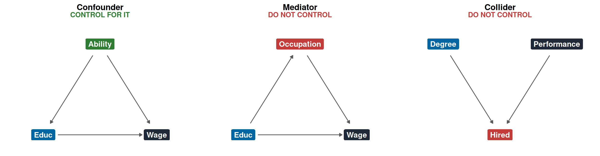
A good control is a confounder
Our goal is usually the causal effect of one variable \(x_1\). The other regressors exist to hold constant the factors that would otherwise contaminate it.
A confounder is a pre-treatment variable correlated with both \(x_1\) and \(y\). Leave it out and \(\hat{\beta}_1\) absorbs its effect, which is Lecture 2’s omitted variable bias.
Example
In estimating the effect of education on wages, innate ability is the classic confounder: it raises schooling and it raises earnings.
Controlling for a proxy such as a test score stops the return to education from being biased upwards.
The validity of a causal estimate rests on choosing the right controls. Including the wrong ones can be worse than including none at all, which is the subject of the next slide.
A bad control is a mediator or a collider
Two kinds of variable induce bias when you control for them.
A mediator lies on the causal pathway from \(x_1\) to \(y\). Controlling for it closes one of the channels through which \(x_1\) acts, so you hold constant part of the very effect you wanted to measure.
A collider is caused by both \(x_1\) and \(y\). Controlling for it manufactures an association between them even when none exists.
Example: a collider
Does a degree (\(x_1\)) raise job performance (\(y\))? A firm hires you if you look promising, and both a degree and raw talent help you get in. Being hired (\(z\)) is caused by both.
Look only at the people the firm hired, and the two can appear negatively related: without a degree you had to be exceptionally good to be hired at all, while a degree gets an average candidate through the door.
Note the equivalence: restricting the sample to those who were hired and adding “was hired” as a control are the same operation. Selecting your sample on a variable is controlling for it.
The three cases as pictures
Arrows point from cause to effect. The question is always the same: should the third variable go into the regression?
The rule of thumb: control for causes of your treatment, never for consequences of it.
Watch the coefficient move
Recall the world from Lecture 2, where we chose \(\beta_0 = 1.5\) and \(\beta_1 = 1.2\). We keep that same return to education, and extend the world with two further forces: experience, and innate ability, which raises both schooling and wages.
So the truth is still that one extra year of education raises wages by 1.2. Watch what happens to educ as we add controls:
Column (1) gives 1.854, far above the true 1.2. Ability is missing, so the education coefficient absorbs the wage premium that really belongs to ability.
Column (2) adds experience, and the coefficient barely moves, from 1.854 to 1.849. Experience is a perfectly valid regressor, but it is uncorrelated with education, so leaving it out never biased anything.
Column (3) adds ability and the coefficient collapses to 1.212, essentially the truth.
The lesson
What removes bias is not more controls, it is the right control.
Adding regressors unrelated to your variable of interest raises the \(R^2\) a little and changes your estimate not at all. Adding a mediator or a collider makes things actively worse.
The bias in column (1) is upward because ability raises both schooling and pay. In general its sign is the product of those two signs, exactly as Lecture 2’s formula said.
Controls are not free
Adding regressors changes the variance of your estimate, and not always for the better.
Variance of the OLS estimator with several regressors
\(SST_j = \sum_i (x_{ij} - \bar{x}_j)^2\) is the total variation in \(x_j\).
\(R_j^2\) is the \(R^2\) from regressing \(x_j\) on all the other regressors.
The new term is \(R_j^2\), and it measures multicollinearity: how much of \(x_j\) is already explained by the other controls. As \(R_j^2\) approaches 1, the denominator shrinks and the variance explodes. The no perfect collinearity assumption is simply \(R_j^2 \neq 1\).
There is a real tension here. A control that is highly correlated with your treatment is often exactly the control you need, and it is also the one that costs you the most precision.
The single \(\hat{\sigma}^2\) in the numerator assumes constant error variance and uncorrelated errors. The second half of this lecture dismantles both.
Testing
Is the number distinguishable from zero?
Our estimates come from a sample, so they are subject to sampling variability. It is entirely possible that the true population relationship is zero and we found a non-zero \(\hat{\beta}_1\) by chance.
Two tools separate signal from noise, and they answer different questions:
The \(t\)-test asks about one coefficient at a time.
The \(F\)-test asks about several coefficients jointly, or about the model as a whole.
The \(t\)-test
The \(t\)-test handles a hypothesis about a single coefficient, most often that the variable has no effect: \(H_0: \beta_j = 0\) against \(H_A: \beta_j \neq 0\).
where \(se(\hat{\beta}_j)\) is the square root of the variance on the previous slide.
It measures how many standard errors the estimate lies from the hypothesized value. Nothing about it is new: it is Lecture 2’s statistic with a multivariate standard error underneath.
The \(F\)-test
The \(F\)-test handles multiple coefficients at once. Its most common use is testing the overall significance of a model.
\(H_0\): none of the explanatory variables affect \(y\), so \(\beta_1 = \beta_2 = \dots = \beta_k = 0\). The model has no explanatory power.
\(H_A\): at least one coefficient is non-zero.
More generally, the \(F\)-test compares a restricted model, in which some coefficients are set to zero under the null, against an unrestricted model in which they are free. A large \(F\)-statistic means the unrestricted model explains substantially more variation, and as usual we read the \(p\)-value.
Where the \(F\)-statistic comes from
Definition: the \(F\) statistic
\[
F = \frac{(SSR_{r} - SSR_{u}) / q}{SSR_{u} / (n - k - 1)}
\]
\(SSR_{r}\): sum of squared residuals from the restricted model, with the null imposed.
\(SSR_{u}\): sum of squared residuals from the unrestricted model.
\(q\): the number of restrictions. Count the equals signs in \(H_0\): for \(H_0: \beta_1 = \beta_2 = 0\), \(q = 2\).
\(n\): observations; \(k\): parameters in the unrestricted model, including the intercept.
The numerator is how much worse the fit gets when you impose the null, per restriction. The denominator scales that by how much unexplained variation there was to begin with.
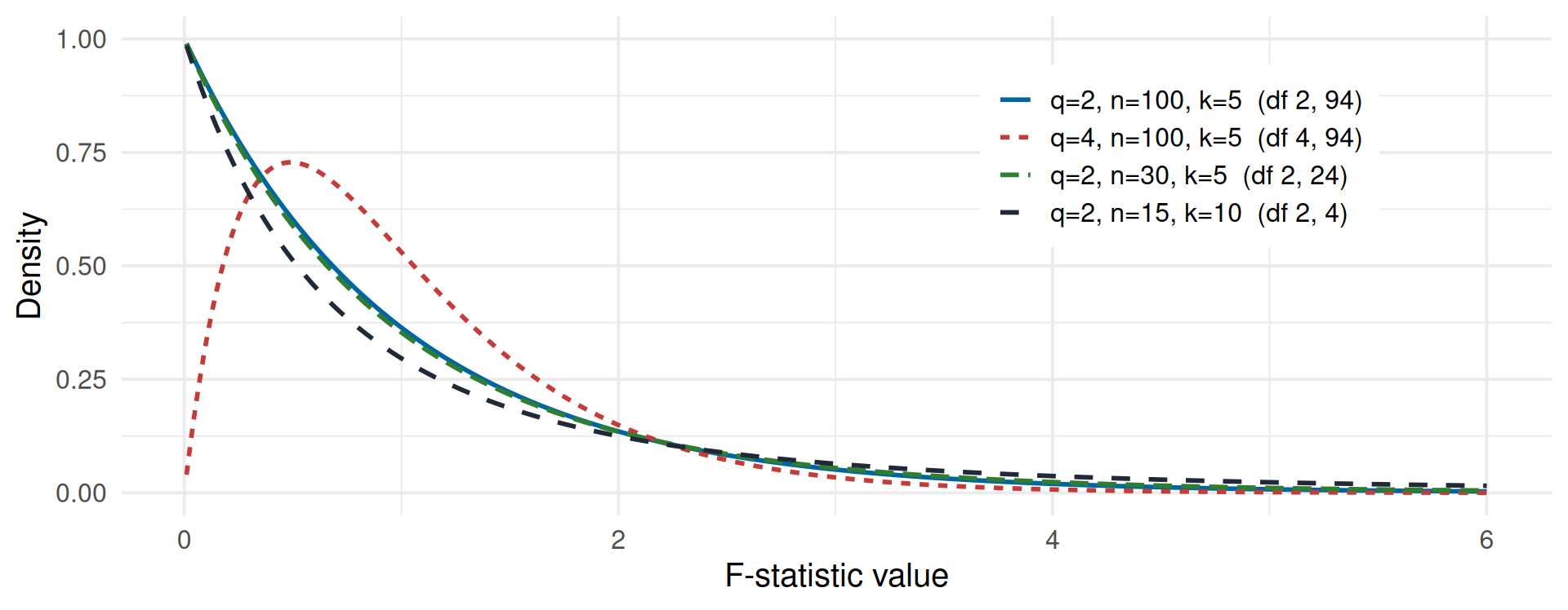
The \(F\) distribution
The distribution takes two degrees-of-freedom parameters, built from \(q\), \(n\), and \(k\). With few observations relative to parameters, the right tail is much heavier, so a much larger \(F\) is needed before anything is surprising.
An \(F\)-test by hand
Take the fully specified model and ask whether experience and ability jointly matter, so \(H_0: \beta_{exper} = \beta_{ability} = 0\) and \(q = 2\).
Rather than call a black box, build the statistic from the formula. It needs two regressions and their sums of squared residuals.
SSR_restricted 24484.3, SSR_unrestricted 17882.5, F 368.4
Code
print(f"p-value {f_dist.sf(f_stat, q, N - k):.3g}")
p-value 6.52e-137
The SSR rises by 37% when we drop the two variables, giving \(F \approx 368\). We reject, and wald() confirms the hand computation exactly.
Two things worth knowing about the \(F\)-test
With one restriction, the \(F\)-test is the \(t\)-test. If \(q = 1\) then \(F = t^2\), and the two always give the same \(p\)-value. Check it on our own output:
The \(F\)-statistic printed in your regression output assumes homoskedasticity. It is built from sums of squared residuals, exactly like the default standard errors. The moment you decide that the classical assumptions fail, which is the subject of the rest of this lecture, that printed \(F\) becomes invalid and you need the robust version, which is what wald() reports once you have set a robust vcov.
\(t\) or \(F\)?
A group of variables can be jointly significant even when no single one of them is individually significant, which is why you need both tools.
\(t\)-test
\(F\)-test
Scope
One coefficient
Two or more coefficients
Typical use
Is this variable significant?
Is this group jointly significant, or the model as a whole?
Null hypothesis
\(H_0: \beta_j = 0\)
\(H_0: \beta_1 = \beta_2 = \dots = 0\)
Statistic
\(t = \hat{\beta}_j / se(\hat{\beta}_j)\)
Compares restricted and unrestricted sums of squares
Example question
Does education affect wages, holding other factors constant?
Do exper and exper^2 jointly affect wages?
The classic case for the \(F\)-test is two highly collinear regressors. Neither can be told apart from zero on its own, yet together they clearly matter.
Dummies and interactions
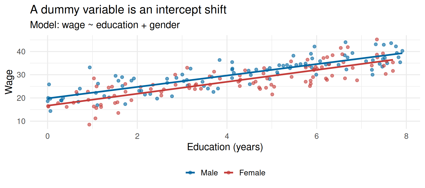
A dummy shifts the intercept
Lecture 2 introduced a dummy on its own. Its power appears once other regressors join it:
Two lines with a different intercept and the same slope. So \(\beta_0\) is the intercept for the reference group, \(\beta_1\) the wage difference between women and men with the same education, and \(\beta_2\) the return to education, which this model forces to be equal for both.
Parallel slopes
The two lines are separated vertically by exactly \(\beta_1\), at every level of education.
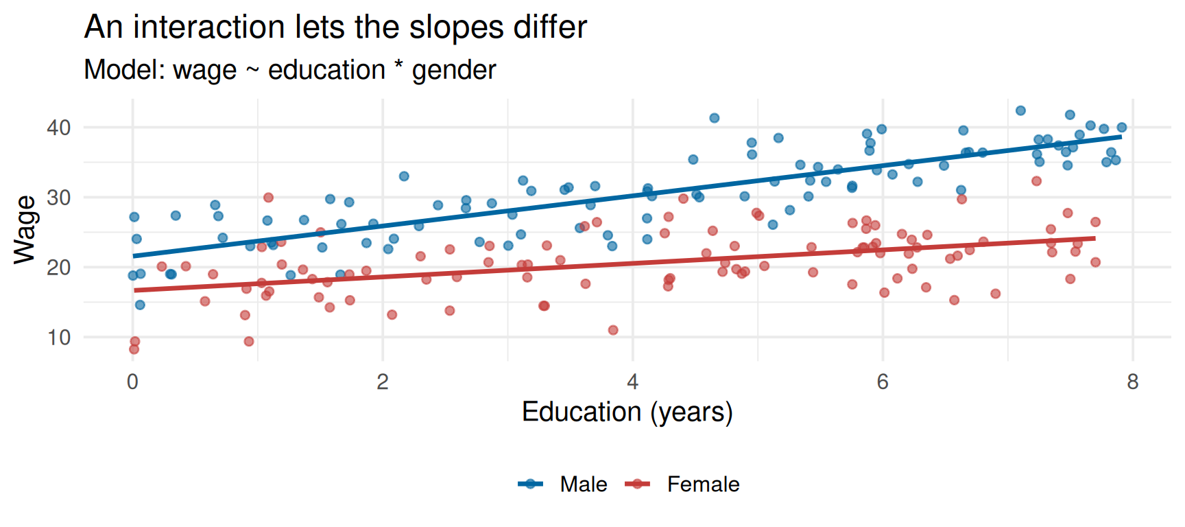
Interactions let the slope differ too
The parallel-slopes model assumes the return to education is identical for men and women. What if it is not?
To let the slope differ, add the product of the dummy and the continuous variable:
So women have intercept \((\beta_0 + \beta_1)\) and slope \((\beta_2 + \beta_3)\).
Reading an interaction
The presence of an interaction changes what the “main effects” mean, which is where most mistakes happen.
\(\beta_2\) is the effect of education for the reference group only, not for everyone.
\(\beta_1\) is the wage difference between women and men when \(Educ = 0\). If zero education never occurs in the data, this number is not interpretable on its own.
\(\beta_3\), the interaction coefficient, is the difference in slopes. It says by how much the return to education differs for women, and it is usually the coefficient of interest.
So the effect of education is \(\beta_2\) for men and \(\beta_2 + \beta_3\) for women.
Different slopes, visually
The lines now converge, so the size of the gap depends on where you stand on the horizontal axis.
The effect is now a function
With an interaction, the effect of a variable is no longer a single coefficient. It is a function of another variable.
Two quantities you may be asked for
The marginal effect of education for women: \[
\frac{\partial E[wage \mid F = 1, Educ]}{\partial Educ} = \beta_2 + \beta_3.
\]
The wage gap between women and men: \[
\begin{aligned}
E[wage \mid F=1] - E[wage \mid F=0]
&= \big[(\beta_0 + \beta_1) + (\beta_2 + \beta_3)Educ\big] - \big[\beta_0 + \beta_2 Educ\big] \\
&= \beta_1 + \beta_3 Educ.
\end{aligned}
\]
The gap is not constant. It depends on the level of education.
This also dictates how you test things. For a different return to education, test \(H_0: \beta_3 = 0\) with a \(t\)-test. For gender having any effect at all, the two lines must coincide, so test \(H_0: \beta_1 = \beta_3 = 0\) jointly with an \(F\)-test.
More than two categories
A categorical variable with \(k\) categories, such as region, cannot simply be coded 1, 2, 3, 4. That would impose an ordering and equal spacing that do not exist.
Instead, create \(k - 1\) binary dummies. Each observation takes the value 1 on its own category’s dummy and 0 on all the others.
The dummy variable trap
You must always omit one category, which becomes the baseline or reference.
Include a dummy for every category and you have perfect multicollinearity: knowing an observation is not in the North, South, or East tells you it is in the West. The model cannot separate effects that are perfectly redundant, and the software will drop one for you or refuse to run.
With West as the baseline: \[
y_i = \beta_0 + \beta_1 \text{North}_i + \beta_2 \text{South}_i + \beta_3 \text{East}_i + \dots + u_i.
\]
Interpreting a set of dummies
The intercept \(\beta_0\) is now the average outcome for the baseline category, with all other regressors at zero.
Each dummy coefficient is the average difference between that category and the baseline, holding other variables constant. It is not that category’s average.
Statistical significance follows the same logic: a significant \(p\)-value on the North dummy says North differs from West, not that it differs from South or East.
Example: predicting wages
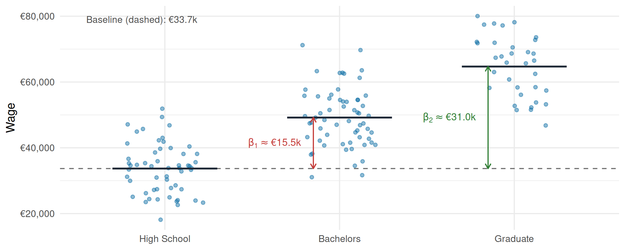
With “High School” as the baseline, suppose \[
\widehat{\text{Wage}}_i = 35{,}000 + 15{,}000 \cdot \text{Bachelors}_i + 30{,}000 \cdot \text{Masters}_i.
\]
High School earns €35,000; Bachelors earn €15,000 more, so €50,000; Masters earn €30,000 more, so €65,000.
Changing the baseline changes nothing that matters
Your choice of baseline changes the interpretation of the individual coefficients, and the coefficients themselves. It does not change what the categorical variable as a whole is doing.
For a set of dummies representing one categorical predictor, the \(F\)-test asks the joint null that all of them are zero: does “Education” have any explanatory power at all?
Whichever category you drop, you are using the same information and explaining the same variation, so the \(R^2\) and the \(F\)-statistic are unchanged. The conclusion about whether education matters never depends on your reference level.
The individual \(t\)-tests are a different matter. Each one tests a specific comparison against the baseline, so changing the baseline changes which comparisons you happen to be testing.
Three categories, visually
Each dummy coefficient is a vertical distance from the dashed baseline, and nothing else.
Reading regression output
Everything on one screen
By now we can read essentially all of the standard output. Here is the fully specified wage regression:
Coefficients.Estimate gives \(\hat{\beta}_0\) through \(\hat{\beta}_3\). Std. Error is \(se(\hat{\beta}_j)\), measuring sampling uncertainty. t value is their ratio, and Pr(>|t|) is the \(p\)-value of the two-sided test against zero.
Goodness of fit. The residual standard error is the SER from Lecture 2, here 2.99, close to the \(\sigma = 3\) we built into the data. The \(R^2\) is 0.64, so the model accounts for about 64% of the variation in wages, against 51% for the simple regression on education alone.
Note what that jump in \(R^2\) does and does not tell you. Fit improved, and the coefficient on education also changed by a third. Only one of those two facts is about credibility.
Interpretation with controls
Every coefficient has an economic interpretation, whatever its statistical significance. The standard error, \(t\)-statistic, confidence interval, and \(p\)-value quantify sampling uncertainty; they do not decide whether a number means anything.
Education:\(\hat{\beta}_1 \approx\) 1.21. Holding experience and ability constant, one more year of education is associated with €1.21 per hour more.
Experience:\(\hat{\beta}_2 \approx\) 0.19. Holding education and ability constant, one more year of experience is associated with €0.19 per hour more.
Ability:\(\hat{\beta}_3 \approx\) 1.98. A one standard deviation higher score is associated with €1.98 per hour more.
A useful habit
Because we built this world, we can check the answers: the true values are 1.2, 0.20, and 2.0, and all three estimates land within about one standard error.
In real data you never get to run this check, which is why the assumptions behind those standard errors matter so much. That is where we go next.
When the default standard error lies
Where the variance comes from
Everything so far has trusted the second column of the output. Now we ask what it assumes.
The variance of the OLS estimator, conditional on the regressors, is
To evaluate that second factor we need assumptions about the errors, and the default output in R and Python imposes two:
Errors are uncorrelated across observations: \(\operatorname{Cov}(u_i, u_j) = 0\) for \(i \neq j\).
Homoskedasticity: the variance is constant, \(\operatorname{Var}(u_i) = \sigma^2\).
This section attacks assumption 2, the next one attacks assumption 1.
A simplification, not a restriction
This whole half uses the single-regressor formulas, and writes \(\operatorname{Var}(\hat{\beta}_1)\) for the conditional variance \(\operatorname{Var}(\hat{\beta}_1 \mid X)\). Every insight carries over unchanged to the multivariate case.
Homoskedasticity, and what it buys
Under homoskedasticity the variance collapses to the formula from Lecture 2:
It is a convenient assumption, and in economic data it is usually false. Heteroskedasticity means the error variance is not constant across observations, and ignoring it makes our inference misleading even though our estimates remain fine.
Same line, different confidence
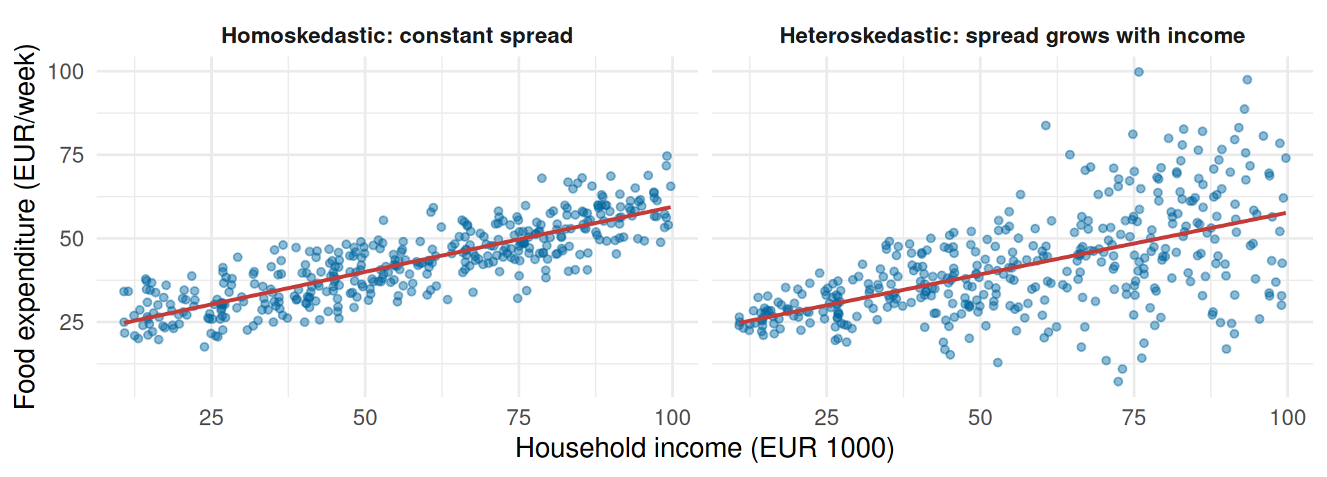
Both panels have the same true line. Only the scatter around it differs.
OLS fits the same line in both cases, and is unbiased in both. What changes is how much confidence we are entitled to have in that line.
The variance under heteroskedasticity
Formally, heteroskedasticity means \(\operatorname{Var}(u_i) = \sigma_i^2\): the variance carries an \(i\) subscript, so it can differ for every observation.
The food expenditure example makes it concrete. Low-income households have limited budgets, so their spending clusters tightly. High-income households have discretion: some spend lavishly, some frugally, and the spread is wide. The error variance grows with income.
With non-constant variance, the true variance of the OLS estimator is
This is not an approximation or a correction. It is what the variance actually is whenever the \(\sigma_i^2\) differ, and the classical formula is the special case in which they do not.
We cannot see \(\sigma_i\), so we use the residual
The obstacle is that we do not know the individual error variances \(\sigma_i^2\).
White’s (1980) insight: use the squared OLS residual \(\hat{u}_i^2\) for each observation as an estimate of its \(\sigma_i^2\). Any single squared residual is a terrible estimate of a single variance, but the sum of them is a consistent estimate of the sum we need.
Its square root is the heteroskedasticity-robust standard error, also called the White or HC standard error. Because it relies on that summation argument, it is a large-sample result.
HC-robust standard errors correct for heteroskedasticity, and for nothing else. They do not correct for serial correlation, and they certainly do not correct for omitted variable bias.
For serial correlation in time series, HAC or Newey-West standard errors are the usual choice. When dependence follows a credible group structure, clustered standard errors are appropriate, which is the next section.
Use them by default
In cross-sectional data heteroskedasticity is the rule, not the exception, and the modern consensus is to use HC-robust standard errors by default.
The cost of using them when errors happen to be homoskedastic is negligible in large samples. The cost of omitting them when they are needed is invalid inference.
Three misconceptions worth killing
“Robust standard errors fix my estimates.” They do not. OLS stays unbiased and consistent under heteroskedasticity; what it loses is efficiency. Robust standard errors fix the inference and leave the estimator alone. Regaining efficiency would need a different method, such as weighted least squares.
“Robust standard errors are always larger.” Also false. They are larger when observations with unusual \(x\) values happen to have large residuals, which is common, but they can easily come out smaller. Robust does not mean conservative; it means correct under weaker assumptions.
“Changing vcov changed my results.” It cannot change \(\hat{\beta}\). The point estimates are identical whichever variance estimator you choose, and only the second column moves. If a coefficient changed, you changed the specification too.
Clustered standard errors
Errors that travel in groups
Now the other default assumption, \(\operatorname{Cov}(u_i, u_j) = 0\). In many economic datasets it is plainly unrealistic: students within schools, individuals within states, firms observed over time.
Unobserved factors at the group level induce correlation among the errors inside that group. This structure is called clustered data.
Before doing any algebra, let us find out how much damage ignoring it actually does.
A world where we know the answer
We build 50 schools of 30 students each, so \(N = 1500\). Each student’s error splits in two, \(u_{gi} = a_g + e_{gi}\): a shock \(a_g\)shared by everyone in school \(g\), plus individual noise \(e_{gi}\).
The share of error variance carried by the shared piece is
\[
\rho_u = \frac{\operatorname{Var}(a_g)}{\operatorname{Var}(a_g) + \operatorname{Var}(e_{gi})} = \operatorname{Corr}(u_{gi}, u_{gj}), \quad i \neq j \text{ in the same school},
\]
so \(\rho_u\) is exactly the intra-cluster correlation of the errors. We set \(\rho_u = 0.5\).
A “policy” is assigned by coin flip to whole schools, and its true effect is exactly zero. A 5% test applied to a true null should reject about 5% of the time. We run 1000 fresh datasets and count.
The simulation in code
One replication builds a fresh world, runs feols once, and returns the estimate with all three standard errors. run_sim repeats that 1000 times and records how often each standard error rejects.
Code
set.seed(2026)# One replication of a world in which the null hypothesis is TRUE.one_replication <-function(cluster_level_x) { G <-50; Ng <-30; rho_u <-0.5 g <-rep(1:G, each = Ng)# Each school gets a shared shock a_g on top of individual noise e_gi. u <-rep(rnorm(G, 0, sqrt(rho_u)), each = Ng) +rnorm(G * Ng, 0, sqrt(1- rho_u))# The policy either varies only across schools, or freely within them. x <-if (cluster_level_x) rep(rbinom(G, 1, 0.5), each = Ng) elserbinom(G * Ng, 1, 0.5) y <-0* x + u # the TRUE effect of x is exactly zero d <-data.frame(y = y, x = x, g = g) m <-feols(y ~ x, data = d, vcov ="iid")c(b =coef(m)["x"],classical =se(m)["x"],hc1 =se(summary(m, vcov ="hc1"))["x"],cr1 =se(summary(m, vcov =~g))["x"])}run_sim <-function(cluster_level_x, reps =1000) { out <-t(replicate(reps, one_replication(cluster_level_x)))colnames(out) <-c("b", "classical", "hc1", "cr1")# Software uses t with G-1 degrees of freedom for clustered tests, N-2 otherwise. cv_n <-qt(0.975, 1500-2); cv_g <-qt(0.975, 50-1)list(reject =c(classical =mean(abs(out[, "b"] / out[, "classical"]) > cv_n),hc1 =mean(abs(out[, "b"] / out[, "hc1"]) > cv_n),cr1 =mean(abs(out[, "b"] / out[, "cr1"]) > cv_g)),mean_se =colMeans(out[, c("classical", "hc1", "cr1")]),true_sd =sd(out[, "b"]) )}sim_cluster <-run_sim(TRUE)sim_individual <-run_sim(FALSE)
The damage
Policy assigned at the school level, true effect zero, nominal significance level 5%:
Standard error used
Rejects a true null
Average SE reported
True sampling sd of \(\hat{\beta}_1\)
Classical (the default)
64.4%
0.052
0.213
HC1 robust
64.6%
0.052
0.213
CR1 clustered
7.5%
0.203
0.213
The default standard error is about 4.1 times too small, and a test that should reject 5% of the time rejects 64% of the time. Compare that with the factor you guessed at the start.
Heteroskedasticity-robust standard errors do not help at all, 64.6% against 64.4%. HC-robust errors fix the diagonal of the variance matrix, and the problem here is entirely off the diagonal. “Robust” is not a general-purpose insurance policy.
The clustered standard error gets close, though not exactly to 5%. We return to why at the end of the section.
The same simulation, one change
Now assign the policy within schools, by flipping a coin for each student separately. Everything else, including \(\rho_u = 0.5\), is unchanged.
Standard error used
Rejects a true null
Average SE reported
True sampling sd of \(\hat{\beta}_1\)
Classical (the default)
5.4%
0.051
0.052
HC1 robust
5.4%
0.051
0.052
CR1 clustered
5.9%
0.051
0.052
Every standard error is now correct, and clustering buys you nothing.
The actual rule
Correlated errors on their own are harmless. The disaster needs correlated errors combined with a regressor that is also correlated within clusters.
Ask yourself not “are my errors clustered?” but “at what level does my treatment vary?”
Notation for clustered data
Let \(g\) index the cluster, such as a school, and \(i\) the individual within it, so an observation is \(gi\):
\[
y_{gi} = \beta_0 + \beta_1 x_{gi} + u_{gi}.
\]
The defining feature of clustered data is the error structure:
\(\operatorname{Cov}(u_{gi}, u_{gj}) \neq 0\) for \(i \neq j\): correlation within a cluster.
\(\operatorname{Cov}(u_{gi}, u_{g'j}) = 0\) for \(g \neq g'\): no correlation between clusters.
Using the standard OLS formula zeroes out all those within-cluster covariance terms. When they are on average positive, which is the common case, we systematically underestimate the variance of \(\hat{\beta}_1\), and our standard errors come out too small.
What each estimator is willing to assume
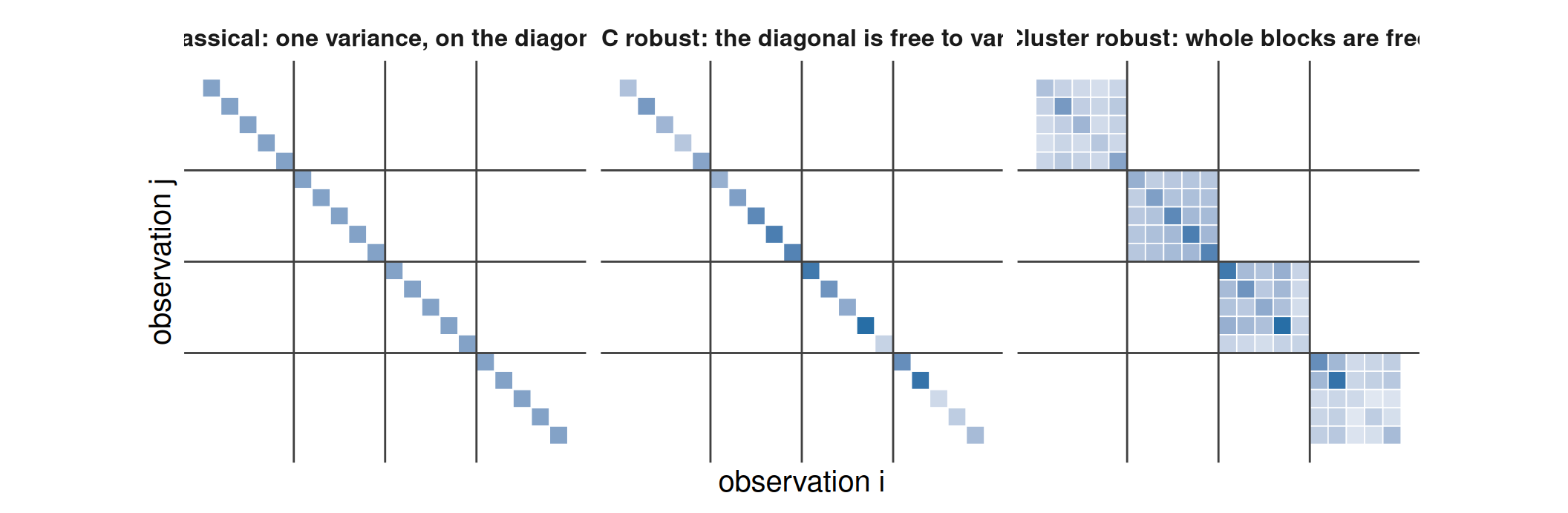
Every one of the three estimators is a statement about which entries of the error covariance matrix \(E[uu']\) may be non-zero. Shaded cells are free; white cells are assumed to be zero.
Reading left to right, each estimator relaxes an assumption rather than adding a correction. Clustering does not “inflate” your standard errors: it stops forcing the off-diagonal blocks to be zero.
Sum inside, square outside
The clustered estimator is computed in four steps.1 Run OLS as usual to get residuals; group them by cluster; for each cluster compute a term capturing the variances and covariances within it; sum those terms across clusters.
The whole difference from the HC estimator fits in one phrase: sum inside, square outside.
HC squares each observation’s contribution, then adds up \(N\) of them.
The clustered estimator adds up the contributions within a cluster first, squares that cluster total, then adds up \(G\) of them.
Squaring after adding is exactly what preserves the cross-products \(\hat{u}_{gi}\hat{u}_{gj}\) that HC throws away.
Effectively this treats each cluster as one larger observation. If observations within a cluster carry very similar information, the cluster contributes less unique information than the same number of independent observations would, which is why the resulting standard errors are typically larger.
where \(\rho_u\) is the intra-cluster correlation of the errors, \(\rho_x\) that of the regressor, and \(\bar{N}_g\) the average cluster size.
The factor is 1, so clustering does nothing, whenever any ingredient is missing: no shared shocks (\(\rho_u \approx 0\)), a regressor varying randomly within clusters (\(\rho_x \approx 0\)), or tiny clusters.
All three large at once is the disaster case, and it describes a great many policy evaluations: a state-level law observed on many individuals per state.
In our simulation \(\rho_u = 0.5\), \(\rho_x = 1\), and \(N_g = 30\), giving \(\sqrt{1 + 0.5 \times 29} = 3.94\). The simulation delivered 4.13.
Why the ratio grows with cluster size
Ask what happens to the average error in a school as we enrol more students:
Only the individual noise averages away. The school-wide shock \(a_g\) never does, because every student carries the same\(a_g\). A school of 1000 students is barely more informative about that school than a school of 30.
The classical formula does not know this. It treats each extra student as a fresh independent draw and keeps shrinking the standard error like \(1/\sqrt{N}\), when precision is really governed by the number of schools.
The gap therefore widens as \(N_g\) grows, and \(\sqrt{1 + \rho_u \rho_x (N_g - 1)}\) measures exactly that: each extra student adds \(N_g - 1\) positive covariance terms that the classical formula sets to zero.
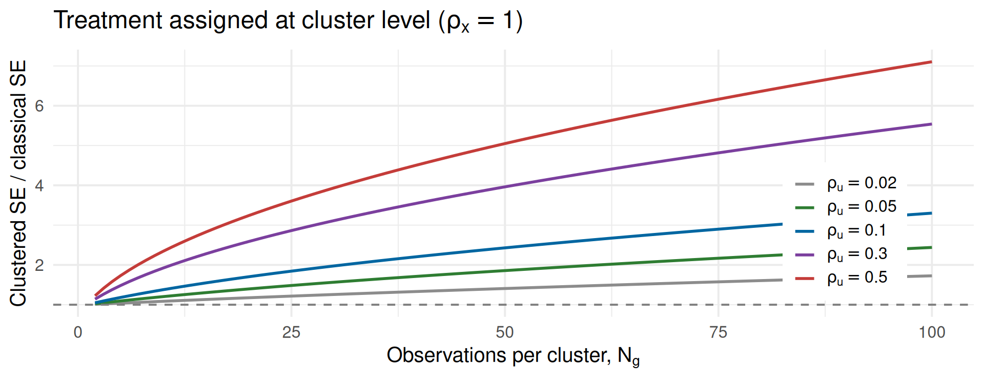
The Moulton factor, visually
Note how little intra-cluster correlation it takes. Even \(\rho_u = 0.05\), which you would never notice by eye, doubles the standard error once clusters contain 60 observations.
Explore it yourself
Treatment varies
Standard error
Mean
Rejects
Classical
—
—
HC1 robust
—
—
CR1 clustered
—
—
True sd of β̂1
—
5% ideal
Moulton factor √(1 + ρuρx(Ng−1)) =
—
300 datasets in which the true effect is zero. Bars are the actual spread of
β̂1; curves are what each standard error claims that spread is.
Set ρu to zero, or let treatment vary within clusters, and all three curves
collapse onto the bars.
When to cluster
The modern answer is a statement about research design, not a hunch about the errors. Cluster when your treatment is assigned at the cluster level, or when your sample was drawn in clusters, as in multi-stage surveys.
Panel data qualify on both counts, since each individual is a cluster of their own repeated observations. That is why this discussion is the last thing we do before the panel lectures.
Clustering because “the data have a group variable in them” is not a reason. As the second simulation showed, if the regressor varies randomly within groups, clustering changes nothing.
The consequence of failing to cluster when you should is severe: standard errors biased downwards, sometimes by a factor of four or more, leaving you overconfident and reporting spurious findings.
At what level should you cluster?
Cluster at the level at which the unobserved components are shared, and at which treatment was assigned.
With students in classrooms within schools, and a policy rolled out by school, cluster on school. This allows for correlation within classrooms and between classrooms in the same school.
Clustering at too fine a level, here the classroom, leaves the between-classroom correlation unaccounted for, so you are back to overconfident standard errors.
The binding constraint in the other direction is that you need enough clusters at whatever level you choose, which is the subject of the next slide.
Three things to remember in practice
Clustering never changes \(\hat{\beta}\). Only the standard errors, \(t\)-statistics, and \(p\)-values move. If your coefficients change when you cluster, you changed something else by accident.
Cluster-robust standard errors need many clusters, not many observations. They are consistent as \(G \to \infty\), not as \(N \to \infty\). A dataset with 500,000 observations in 12 states has 12 clusters, and its clustered standard errors are still biased downwards. That is why our simulation rejected 7.5% of the time rather than exactly 5%, even with \(G = 50\).
With few clusters, below roughly 40, use the wild cluster bootstrap. In R, fwildclusterboot::boottest(); in Python, pf.feols(...).wildboottest(reps = 9999, param = "x", cluster = "cluster_variable").
Clustering in software
Like HC-robust standard errors, clustered standard errors must be requested explicitly:
feols changes its default the moment you add fixed effects. Writing feols(y ~ x | firm, data = df) clusters on firm automatically, without you asking for it.
Always read the vcov line that fixest prints under the coefficient table, rather than assuming. Better still, set vcov yourself so the choice is visible and deliberate.
Takeaways
What did we learn?
Multiple regression holds other measured factors constant, which is how we act on Lecture 2’s diagnosis.
A good control is a confounder. A mediator or a collider makes the estimate worse, and selecting your sample on a variable is the same as controlling for it.
The right control removes bias; more controls do not. Column (2) proved it by changing nothing.
Controls cost precision through \(R_j^2\), and the most useful control is often the most expensive one.
The \(t\)-test handles one coefficient, the \(F\)-test several; with one restriction they coincide, since \(F = t^2\).
An interaction makes the effect a function of another variable, so “the effect” is no longer a single number.
Default standard errors assume constant variance and uncorrelated errors. Both routinely fail.
HC-robust errors relax the first; cluster-robust errors relax the second. Neither changes \(\hat{\beta}\), and neither fixes bias.
Exit questions
Be able to answer these without looking back:
Adding experience changed the education coefficient by almost nothing. Why?
Why is controlling for a collider harmful when the collider is correlated with both variables?
When are a \(t\)-test and an \(F\)-test guaranteed to give the same \(p\)-value?
In an interacted model, what does the coefficient on the dummy alone mean?
Our simulation had \(\rho_u = 0.5\) throughout, yet clustering mattered in one design and not the other. What differed?
You have 500,000 observations in 12 states, and the policy varies by state. What is your effective sample size for inference?
Answers to the exit questions
Why experience did nothing. Bias is \(\beta_2 \delta_1\), and experience is uncorrelated with education, so \(\delta_1 \approx 0\). A valid control that is orthogonal to the treatment cannot have been biasing anything.
Why a collider harms. It is a consequence of both variables, not a cause. Conditioning on a common effect creates an association between its causes where none existed.
When \(t\) and \(F\) agree. When there is exactly one restriction, \(q = 1\), in which case \(F = t^2\) identically.
The dummy in an interacted model. The group difference evaluated at zero on the interacted variable. If zero is outside the data, it is not interpretable on its own.
What differed between the designs.\(\rho_x\). With treatment assigned to whole schools \(\rho_x = 1\); assigned within schools, \(\rho_x \approx 0\), and the Moulton factor collapses to 1.
Effective sample size. 12. Cluster-robust inference is consistent in the number of clusters, so those clustered standard errors are still biased downwards, and this is a case for the wild cluster bootstrap.
Looking ahead
Controls only work for confounders we can measure. Ability was observable here only because we built the world.
Lecture 4 gets a way to control for an entire class of confounders nobody can measure, as long as they do not change over time.
Appendix: cluster-robust SEs
Setting the scene
This appendix derives the cluster-robust formula we used in the lecture. There is no new economics here: it is the bookkeeping that shows where the formula comes from, and why it takes the odd “sum inside, square outside” shape.
The setting. There are \(G\) clusters, indexed by \(g\), and cluster \(g\) holds \(N_g\) observations indexed by \(i\). As in the main text we keep a single regressor:
The assumption. Errors may be correlated in any way within a cluster, but not at all across clusters:
\[
\operatorname{Cov}(u_{gi}, u_{gj}) \ \text{ unrestricted}, \qquad \operatorname{Cov}(u_{gi}, u_{g'j}) = 0 \ \text{ for } g \neq g'.
\]
Bread and meat
Every variance formula in this section has the same bread and meat shape: a factor built only from the \(x\)’s, multiplying a term built from the errors.
We reach the answer in three steps:
Write \(\operatorname{Var}(\hat{\beta}_1)\) as bread times meat.
Split the meat cluster by cluster, which is where the covariances survive.
Replace the unknown errors \(u_{gi}\) by the observed residuals \(\hat{u}_{gi}\).
Colours used on the slides that follow
\(\color{#0066a1}{\textbf{Blue}}\): the bread, \(\left(\sum (x_{gi} - \bar{x})^2\right)^{-2}\). Identical in the classical, HC and clustered estimators, so it is never the interesting part.
\(\color{#2e7d32}{\textbf{Green}}\): the within-cluster sum, the “sum inside” step that creates clustering.
\(\color{#c43c39}{\textbf{Red}}\): the within-cluster covariance terms, precisely what the classical and HC estimators set to zero.
Expressing the variance
We express \(\operatorname{Var}(\hat{\beta}_1)\) in a form that recognises the cluster structure:
The blue factor is the bread, and it is now fixed for the rest of the derivation. In the final line we only re-indexed: summing over all \(N\) observations is the same as summing within each cluster and then over clusters.
Splitting the meat
Restating the result, with the meat we still have to work on:
The black line is all the HC estimator keeps. The red line is the entire difference, and it is what a classical or HC standard error silently sets to zero.
From errors to residuals
We cannot compute the true variance, because the errors \(u_{gi}\) are unknown. We estimate it from the OLS residuals \(\hat{u}_{gi} = y_{gi} - \hat{y}_{gi}\).
Define a score for each observation, \(s_{gi} = (x_{gi} - \bar{x})\hat{u}_{gi}\). It is built from the residual, which we observe, not the error, which we never do. Let the cluster total be
This green object is the sample counterpart of the green term on the previous slides.
Squaring after summing
The single-cluster variance can be written as an expected squared sum, \(E\left[ \left( \sum_{i} (x_{gi} - \bar{x})u_{gi} \right)^2 \right]\).1
A natural estimator is the squared cluster total, \(\color{#2e7d32}{(s_g)}^2\). Squaring after summing is the step that keeps the red covariance terms: expanding \((s_{g1} + \dots + s_{gN_g})^2\) produces every cross-product \(s_{gi}s_{gj}\).
Summing over clusters estimates the meat in Equation 1:
The blue bread is the same in both. The only difference is where the summation sits relative to the square.
HC squares each observation on its own and adds \(N\) of them, which assumes independence. The clustered estimator sums green inside first, squares that cluster total, and adds \(G\) of them. Expanding the square recreates every \(\color{#c43c39}{\text{red covariance term}}\) without ever estimating one individually.