Empirical Economics

Lecture 5: Panel Data II

Outline

Course Overview

Introduction to Econometrics and Data
Linear Model I
Linear Model II
Panel Data I
Panel Data II

What do we do today?

This is the second of two lectures on panel data. It builds on fixed effects and first differences, within and between variation, strict exogeneity, and clustered standard errors.

We define pooled OLS and ordinary random effects and state what each assumes. We then study quasi-demeaning and correlated random effects (the Mundlak model), which allows the person effect to correlate with the time-varying regressors.

In Lecture 4, fixed effects removed time-invariant confounders by comparing each person with himself over time. Today we study estimators that also compare different people and the assumptions needed to use those comparisons.

The corresponding reading is Wooldridge, Sections 13.1, 13.2, 14.2 and 14.3.

What should you be able to do?

By the end of this lecture, you should be able to:

State what pooled OLS assumes, and why it still needs clustered standard errors.
Explain the random-effects assumption and why it is stronger than the fixed-effects one.
Write down the quasi-demeaning parameter \(\theta\) and place pooled OLS, RE and FE on it.
Carry out and interpret the Breusch–Pagan LM and Hausman tests.
Estimate and interpret the Mundlak model as a robust alternative to FE.
Justify a choice of panel estimator on economic grounds as well as on test results.

Guiding questions

Is union membership associated with higher wages?
What is the return to a year of schooling?

We observe 545 young men in each of 8 years, 1980 to 1987 (Vella and Verbeek, 1998). The outcome is the log of the hourly wage. We estimate a wage regression with union membership and years of schooling as explanatory variables.

Prediction

Lecture 4 gave you a fixed-effects estimator. Write down which of these two questions it can answer and which it cannot.

We return to your answer later in the lecture.

What fixed effects cannot estimate

Within and between variation by regressor

Variable	Between-person SD	Within-person SD
educ	1.748	0.000
black	0.320	0.000
hisp	0.363	0.000
union	0.329	0.195
married	0.377	0.258
exper	1.655	2.449

The within-person standard deviation of education, being black, and being Hispanic is exactly zero. Nobody in this panel returns to school, and nobody changes ethnicity.

Consequences of zero within variation

Lecture 4 showed that the within transformation subtracts each person’s own mean, so a regressor that never moves within a person satisfies \(z_i - \bar z_i = 0\) and drops out of the equation. In the dummy-variable version of the same estimator, \(z_i\) is perfectly collinear with the person fixed effect, so the two cannot be separated.

The consequence is one of identification: the return to schooling is not identified by a comparison of a person with himself, because that comparison holds schooling fixed.

Answer to the prediction

Question 1 is answerable by fixed effects: 24.4% of person-years are union, and men move in and out of unions.

Question 2 is not. Fixed effects drops educ from the estimation.

Answering question 2 therefore requires an estimator that retains the between-person comparison. The rest of the lecture states what such an estimator assumes.

Pooled OLS

The pooled OLS model

Pooled OLS applies ordinary least squares to all \(NT\) observations at once, without using the panel structure:

\[ y_{it}=\beta_0+\beta_1x_{1it}+\cdots+\beta_kx_{kit}+v_{it}, \qquad v_{it}=\alpha_i+u_{it}. \]

The individual effect is contained in the composite error \(v_{it}\), which OLS treats as noise.

Nothing is demeaned and nothing is differenced, so a time-invariant \(z_i\) remains in the equation and its coefficient can be estimated.

Consistency and unbiasedness

This is the distinction Lecture 4 drew for fixed effects, applied here.

Two different requirements

Pooled OLS is consistent as \(N\to\infty\) under contemporaneous exogeneity of the composite error, \[E(v_{it}\mid x_{it}) = 0.\]

Pooled OLS is unbiased under strict exogeneity of the composite error, \[E(v_{it}\mid x_{i1},\ldots,x_{iT}) = 0.\]

Both require \(E(\alpha_i \mid x_{it}) = 0\), because \(\alpha_i\) is part of \(v_{it}\). This is the requirement that fixed effects avoids making.

What the consistency assumption means

Compared with fixed effects, the main additional requirement for pooled OLS consistency concerns the person effect. Assuming \(E(u_{it}\mid x_{it})=0\), consistency requires

\[E(\alpha_i\mid x_{it})=0.\]

In our wage panel, \(\alpha_i\) includes persistent unobserved determinants of wages, such as ability. The assumption says that the average person effect is zero at every combination of schooling, union status, and the other included regressors.

Example: schooling and ability

Suppose men with greater unobserved ability obtain more schooling and earn higher wages. Then average ability differs by schooling level, even after accounting for the other regressors, so \(E(\alpha_i\mid x_{it})\neq 0\).

The pooled OLS schooling coefficient then partly reflects differences in ability. A larger sample does not remove this bias.

The composite error is serially correlated

Even when pooled OLS is consistent, its standard errors are not. Because the same \(\alpha_i\) appears in every period for person \(i\),

\[ \operatorname{Cov}(v_{it},v_{is}) =\operatorname{Cov}(\alpha_i+u_{it},\alpha_i+u_{is}) =\operatorname{Var}(\alpha_i) =\sigma^2_\alpha, \qquad t \neq s, \]

while \(\operatorname{Var}(v_{it})=\sigma^2_\alpha+\sigma^2_u\), so that

\[ \operatorname{Corr}(v_{it},v_{is})=\frac{\sigma^2_\alpha}{\sigma^2_\alpha+\sigma^2_u}. \]

Whenever \(\sigma^2_\alpha>0\), observations on the same person are positively correlated in every pair of periods. We will use this correlation twice more today: once to build the random-effects estimator, and once to test for it.

Clustering revisited

Lecture 3’s rule sets the cluster level by the level at which the treatment varies. Union status varies person by person and persists over time, so we cluster on the person.

Coefficient	Estimate	Default SE	Clustered SE
union	0.1801	0.0171	0.0276
educ	0.0994	0.0047	0.0092

Clustering leaves both coefficients untouched and raises the standard error on union by 61%, and the one on educ by 97%. The default standard errors were counting 8 observations per man as 8 independent pieces of evidence.

Pooled OLS on the wage panel

	Default SEs	Clustered by person
* p < 0.1, p < 0.05, * p < 0.01
Controls for experience and its square included but not shown.
Union member	0.180***	0.180***
	(0.017)	(0.028)
Years of education	0.099***	0.099***
	(0.005)	(0.009)
Married	0.108***	0.108***
	(0.016)	(0.026)
Black	-0.144***	-0.144***
	(0.024)	(0.050)
Num.Obs.	4360	4360
R2	0.187	0.187

Union membership is associated with 18.0 log points, which by Lecture 2’s log-level interpretation is \(e^{0.180}-1\), or 19.7%, higher wages. Whether that association is a causal union effect is the question the rest of the lecture addresses.

Random effects

The between estimator

Consider first the comparison that fixed effects discards. Collapse each man to his eight-year averages and regress those averages on each other:

\[ \bar y_i = \beta_0 + \beta_1 \bar x_{1i} + \cdots + \gamma_1 z_{1i} + \cdots + (\alpha_i + \bar u_i). \]

This is the between estimator: one observation per person, no within variation at all.

Estimator	Union premium	Return to schooling
Between	0.271	0.095
Pooled OLS	0.180	0.099
Fixed effects	0.082	not identified

The between estimate of the union premium is 3.30 times the fixed-effects one. Pooled OLS lands between them, because it uses both comparisons at once.

The random-effects assumption

Random effects uses both comparisons, under the following assumption:

The random-effects assumption

\[ E\!\left(\alpha_i \mid x_{i1},\ldots,x_{iT}\right)=0. \]

The unobserved individual effect is uncorrelated with the entire history of the regressors.

As in the pooled OLS example, this assumption fails if average unobserved ability differs by schooling level after accounting for the other regressors.

The assumption is stronger than the fixed-effects one. Fixed effects allows \(\alpha_i\) to correlate with the regressors; random effects rules that correlation out.

Random effects is consistent under the same condition as pooled OLS. The two differ in efficiency, which the next slide sets out.

Quasi-demeaning

The error correlation is \(\sigma^2_\alpha/(\sigma^2_\alpha+\sigma^2_u)\), so generalized least squares can remove it. GLS subtracts a fraction \(\theta\) of each person’s mean:

\[ y_{it}-\theta\bar y_i =\beta_1\left(x_{1it}-\theta\bar x_{1i}\right)+\cdots+\left(v_{it}-\theta\bar v_i\right), \qquad \theta=1-\sqrt{\frac{\sigma^2_u}{\sigma^2_u+T\sigma^2_\alpha}}. \]

Averaging over \(T\) periods reduces the variance of the temporary error to \(\sigma^2_u/T\) but leaves the person effect unchanged, so a larger \(T\) or \(\sigma^2_\alpha\) calls for more demeaning. The square root converts the variance ratio into a standard-deviation ratio, giving the retained fraction \(1-\theta\) that makes the transformed errors uncorrelated across periods.

The estimator family indexed by \(\theta\)

\(\theta=0\): subtract nothing. This is pooled OLS.
\(\theta=1\): subtract the whole mean. This is fixed effects.
\(0<\theta<1\): random effects, between the two.

What \(\theta\) is in our data

Component	Value
Idiosyncratic, \(\hat\sigma^2_u\)	0.123
Individual effect, \(\hat\sigma^2_\alpha\)	0.105
Implied \(\hat\theta\)	0.643

With \(T=8\) and roughly equal variance components, \(\hat\theta = 0.643\). Random effects subtracts 64% of each man’s mean, placing it that far from pooled OLS towards fixed effects, so its estimates should lie near the fixed-effects ones without coinciding with them.

\(\theta\to 0\) as \(\sigma^2_\alpha\to 0\), and \(\theta\to 1\) as \(T\to\infty\). With enough periods per person, random effects and fixed effects converge.

Estimating the temporary-error variance

Fit the within regression of demeaned log wages on demeaned regressors. Subtracting each man’s mean removes \(\alpha_i\); the remaining residual variation estimates \(\sigma^2_u\).

Square and sum all residuals, then divide by \(NT-N-k=3811\) residual degrees of freedom, with \(k=4\) estimated slopes:

\[\hat\sigma^2_u=\frac{\sum_i\sum_t\hat u^2_{it}}{NT-N-k} =\frac{470.20}{3811} \approx 0.123.\]

Estimating the person-effect variance

Regress each man’s eight-year mean log wage on his mean regressors. The 545 residuals \(\hat e_i\) estimate the combined error \(\alpha_i+\bar u_i\).

The between residual variance is \(\hat\sigma^2_b=\sum_i\hat e_i^2/537\approx 0.121\). Averaging reduces the temporary-error contribution to \(\hat\sigma^2_u/T\approx 0.015\), so subtract it:

\[\hat\sigma^2_\alpha=\hat\sigma^2_b-\frac{\hat\sigma^2_u}{T} \approx 0.105.\]

Four estimates of one coefficient

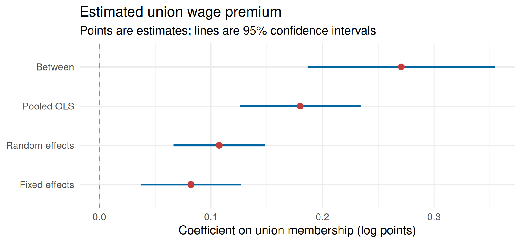
The four estimators differ only in how much between-person variation they use, from all of it to none. No information was added to the data; the between comparison was progressively removed.

Identification of \(\gamma\) and efficiency

Random effects can estimate the coefficient on a time-invariant regressor, because it never fully removes the between comparison.

Random effects is also more efficient than fixed effects when its assumption holds, because it uses both sources of variation instead of one.

Inconsistency when the assumption fails

If \(\operatorname{Cov}(\alpha_i,x_{it})\neq 0\), random effects is inconsistent, and the bias does not shrink with more data. This is Lecture 2’s omitted variable bias, entering through the between comparison that fixed effects removes.

The efficiency gain holds only under the assumption, and the inconsistency arises whenever the assumption fails.

Standard errors for random effects

The efficiency claim rests on more than the exogeneity assumption. GLS is the efficient estimator only if \(u_{it}\) is homoskedastic and serially uncorrelated after the individual effect is accounted for.

In wage data it is neither: wages are persistent for reasons beyond a fixed personal endowment.

So we report random effects with standard errors clustered by person, for the same reason we did it for pooled OLS in Lecture 3’s framework. The GLS transformation handles the part of the serial correlation we modelled; clustering handles the part we did not.

Choosing between the estimators

What economics implies about \(\alpha_i\)

In Lectures 2 and 3 we worked with a data-generating process in which unobserved ability raised both schooling and wages, and the resulting bias could not be removed because ability was unmeasured.

The same structure applies here. The person effect \(\alpha_i\) contains ability, ability is correlated with educ, and it is plausibly correlated with union membership as well.

Retrieval question

Given that, should the random-effects assumption \(E(\alpha_i\mid x_i)=0\) hold or fail in this panel?

What do you therefore expect a test of it to report?

Economic reasoning answers the question before any test is run, and a specification test that agrees with it confirms an argument already made.

The Hausman test

Under strict exogeneity, \(\hat\beta_{FE}\) is consistent whether or not \(\alpha_i\) correlates with \(x\). The estimator \(\hat\beta_{RE}\) is consistent and efficient if \(\alpha_i\) and \(x\) are uncorrelated, and inconsistent if they are correlated.

If the random-effects assumption holds, the two estimators target the same parameter and differ only by sampling noise. If it fails, only the fixed-effects estimator remains consistent for \(\beta\). The Hausman test compares the two sets of estimates on that basis.

The Hausman statistic

For a single coefficient, the statistic is the squared difference between the two estimates, scaled by the difference between their variances:

\[ H=\frac{\left(\hat\beta_{FE}-\hat\beta_{RE}\right)^2} {\operatorname{Var}(\hat\beta_{FE})-\operatorname{Var}(\hat\beta_{RE})} \;\sim\;\chi^2(1). \]

With several coefficients the same construction gives \(\chi^2(k)\), where \(k\) counts the regressors that both estimators identify: the time-varying ones.

The Hausman test on the wage panel

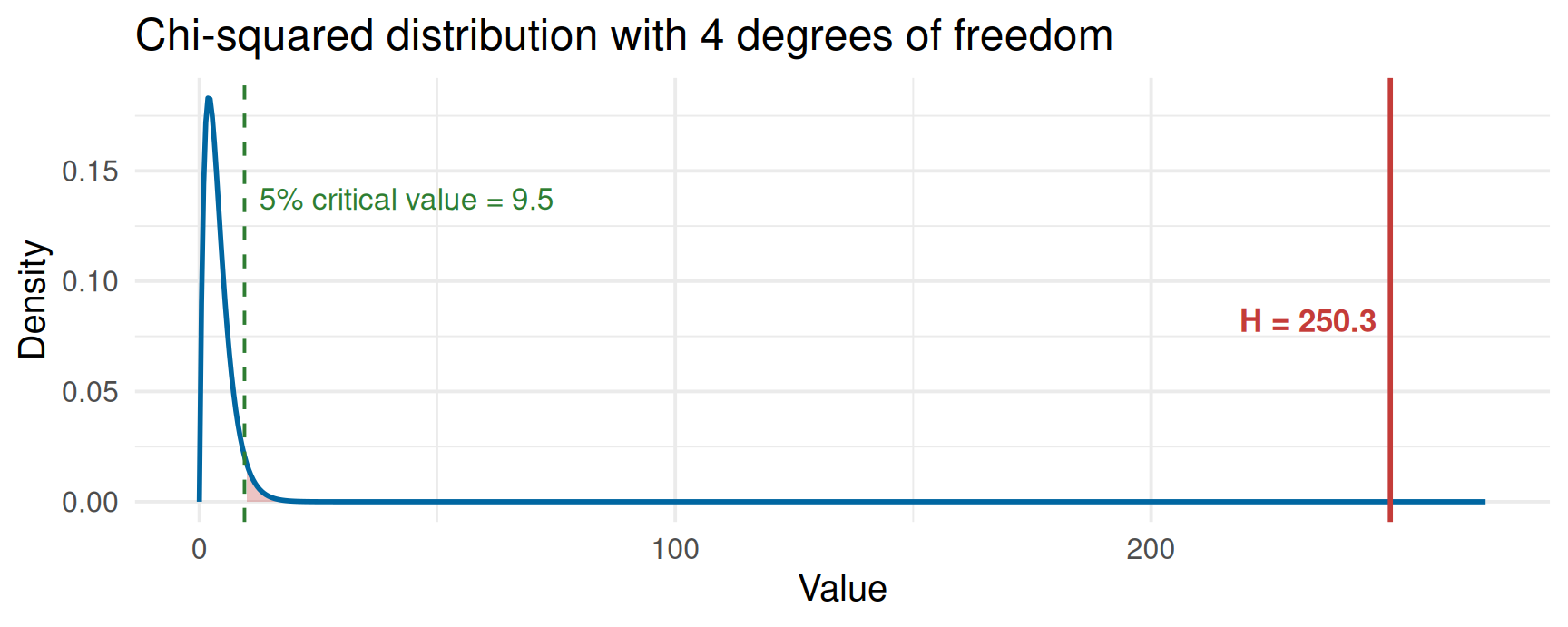
\(H=250.3\) against a 5% critical value of 9.5. We reject at any conventional level, which is what the preceding argument predicted. The fixed-effects estimator is the consistent one here.

What the Hausman test cannot tell you

Two limitations

Failing to reject is not evidence that the assumption holds. The test can be underpowered, and Lecture 2’s warning applies unchanged: the exogeneity of an unobservable cannot be verified from data. Non-rejection means only that no violation was detected.

The classical statistic assumes random effects is efficient under \(H_0\). That requires \(u_{it}\) to be homoskedastic and serially uncorrelated, which is false for wages. When it fails, \(\operatorname{Var}(\hat\beta_{FE})-\operatorname{Var}(\hat\beta_{RE})\) need not be positive, and the statistic can come out negative.

The Mundlak test permits clustered inference.

Correlated random effects

Mundlak’s approach allows \(\alpha_i\) to correlate with the regressors and models that correlation explicitly. Write

\[ \alpha_i=\psi_0+\psi_1\bar x_{1i}+\cdots+\psi_k\bar x_{ki}+c_i, \]

and substitute back. The estimating equation includes each person’s own means as extra regressors:

\[ y_{it}=\beta_0+\beta_1x_{1it}+\cdots+\beta_kx_{kit} +\gamma z_i +\psi_1\bar x_{1i}+\cdots+\psi_k\bar x_{ki}+c_i+u_{it}. \]

The Mundlak specification

Include the person mean of every time-varying regressor, including transformed terms such as \(x_{it}^2\). Time-invariant regressors already equal their own means, so adding their means would create perfect collinearity.

Within and between coefficients in Mundlak

Rewrite the time-varying part of the equation as

\[ x_{it}'\beta+\bar x_i'\psi =(x_{it}-\bar x_i)'\beta+\bar x_i'(\beta+\psi). \]

The coefficient \(\beta\) describes within-person changes. The coefficient \(\beta+\psi\) describes between-person differences, conditional on the time-invariant controls.

In this balanced linear panel, including all the person means reproduces the FE slopes on the time-varying regressors. This does not require the ordinary RE restriction \(\psi=0\).

Using correlated random effects

Use FE or Mundlak when the person effect may correlate with the time-varying regressors. Mundlak also reports coefficients on time-invariant variables; their causal interpretation requires an additional assumption about the remaining person effect.

Correlated random effects on the wage panel

	Fixed effects	Mundlak (CRE)
* p < 0.1, p < 0.05, * p < 0.01
Both clustered by person. Experience terms and their means included, not shown.
Union member	0.082***	0.082***
	(0.023)	(0.023)
Married	0.045**	0.045**
	(0.021)	(0.021)
Years of education		0.095***
		(0.011)
Person mean of union		0.189***
		(0.048)
Person mean of married		0.098**
		(0.045)
Num.Obs.	4360	4360

The coefficients on the time-varying regressors are identical to the fixed-effects ones to four decimals, and educ is estimated, which fixed effects cannot do.

The joint test of the person means gives \(F=7.18\) on \(4\) and \(544\) degrees of freedom, with \(p<0.001\). We reject the ordinary RE restriction using person-clustered inference.

Testing the ordinary RE restriction

Within the Mundlak specification, ordinary RE imposes

\[H_0:\psi_1=\cdots=\psi_k=0.\]

Test the person-mean coefficients jointly with an F test and standard errors clustered by person. The test does not require ordinary RE to be efficient under the null.

Rejection supports retaining the person means and using FE or Mundlak for the time-varying slopes. It does not test strict exogeneity of \(u_{it}\) or the identifying assumption for a time-invariant regressor.

Non-rejection means that this test detected no violation of the restriction. It does not establish that the individual effect is unrelated to every regressor.

Schooling in correlated random effects

The joint test rejects excluding the person means. Correlated random effects is a reasonable specification here: it includes those means and reproduces the fixed-effects estimates for the time-varying regressors.

Schooling does not change within a person, so fixed effects cannot estimate its coefficient. Correlated random effects estimates it by comparing men with different schooling, conditional on their regressor means and other controls.

In this regression, an additional year of schooling is associated with about 9.9% higher wages, holding those controls constant.

Interpreting the schooling coefficient

A causal interpretation requires the remaining person effect \(c_i\) to be unrelated to schooling after conditioning on the person means and other regressors. If unobserved ability still differs by schooling level after those controls, the coefficient still contains ability bias.

Pooled OLS or random effects?

The remaining comparison does not concern identification.

Both estimators require the same assumption about \(\alpha_i\), so the open question is whether there is an individual effect worth modelling. If \(\sigma^2_\alpha=0\), the composite error \(v_{it}=\alpha_i+u_{it}\) reduces to \(u_{it}\): nothing persists within a person, and pooled OLS is already the efficient estimator.

That is a hypothesis about a variance, and it has its own test.

The Breusch–Pagan LM test

The Lagrange multiplier test of Breusch and Pagan (1980) compares two cases. Under \(H_0:\sigma^2_\alpha=0\) there is no individual effect and pooled OLS is efficient. Under \(H_1:\sigma^2_\alpha>0\) a person’s errors share a persistent component, so they are correlated across periods and GLS improves on OLS.

Run pooled OLS, keep its residuals \(\hat v_{it}\), and compare each person’s summed residuals with their individual ones:

\[ LM=\frac{NT}{2(T-1)} \left[\frac{\sum_i\left(\sum_t \hat v_{it}\right)^2}{\sum_i\sum_t \hat v_{it}^2}-1\right]^2 \;\sim\;\chi^2(1). \]

Under \(H_0\) a person’s residuals are as likely to cancel as to reinforce, the ratio in brackets is about 1, and \(LM\) is near zero. A persistent \(\alpha_i\) pushes the residuals of one person to the same side, the ratio grows, and the statistic with it.

The LM test on the wage panel

On our data, \(\chi^2=3217\) against a 5% critical value of 3.84, so \(p<0.001\): there is an individual-effect variance component, and GLS improves on pooled OLS.

The test concerns efficiency only. Pooled OLS and random effects are both inconsistent when \(\alpha_i\) is correlated with the regressors, and the LM test does not examine that condition.

A caveat on the LM test

\(\sigma^2_\alpha=0\) sits on the boundary of the parameter space, since a variance cannot be negative. The usual two-sided \(\chi^2\) approximation is therefore not exact; the one-sided version (type = "honda") is the sharper test.

Consistency by estimator

Assume strict exogeneity of \(u_{it}\) and a correctly specified linear model. The table concerns \(\beta\) on time-varying regressors in this balanced panel.

Estimator	\(\alpha_i\) uncorrelated with \(x_i,z_i\)	\(\alpha_i\) correlated with \(x_i\)
Pooled OLS	Consistent	Generally inconsistent
Ordinary RE	Consistent	Generally inconsistent
FE	Consistent	Consistent
Mundlak (CRE)	Consistent	Consistent, same slopes as FE

FE absorbs time-invariant regressors. Mundlak estimates their coefficients from between-person variation; consistency of \(\gamma\) also requires the residual person effect \(c_i\) to be unrelated to \(z_i\) conditional on the included controls.

Efficiency and inference

Under the ordinary RE restriction and homoskedastic, serially uncorrelated \(u_{it}\), GLS can use between-person information to estimate \(\beta\) more efficiently than FE.

Mundlak estimates separate within and between coefficients. Its time-varying slopes equal FE in this balanced panel, so it does not automatically retain ordinary RE’s efficiency gain for those slopes.

Report person-clustered standard errors for pooled OLS, ordinary RE, FE and Mundlak. Clustering permits within-person dependence; it does not remove omitted variable bias.

Does the error process favour FE or FD?

One diagnostic from Lecture 4 remains. If the level errors \(u_{it}\) are serially independent, differencing induces \(\operatorname{Corr}(\Delta u_{it},\Delta u_{i,t-1})=-0.5\); if instead the levels follow a random walk, the differences are uncorrelated and the benchmark is \(0\).

Regressing the first-difference residuals on their own within-person lag gives -0.396, with a 95% interval of [-0.438, -0.354].

The estimate differs from both benchmarks, so the level errors are neither serially independent nor a random walk. The comparison concerns relative efficiency under a given error process. Both estimators rest on the same identifying assumption, so the diagnostic says nothing about their relative credibility.

A workflow for choosing an estimator

Recommended steps

Compare specifications. Report pooled OLS, ordinary RE, FE, Mundlak and FD side by side.
Cluster at the level at which the treatment varies. This changes inference and leaves the coefficients unchanged.
Use the LM test to check whether there is an individual effect worth modelling, keeping in mind that it says nothing about identification.
Use the clustered Mundlak test to assess the restriction excluding the person means. Predict the answer from economics first.
Decide on economic grounds. Prefer FE or Mundlak when \(\alpha_i\) plausibly correlates with time-varying regressors. Justify a time-invariant coefficient separately.

Lecture 4 noted that no mechanical test-and-choose rule exists. These tests supply evidence, and the choice between estimators is argued.

Comparing the wage estimates

	Pooled OLS	Ordinary RE	FE	Mundlak	FD
* p < 0.1, p < 0.05, * p < 0.01
Person-clustered SEs. Experience controls included; Mundlak also includes all four person means.
Union member	0.180***	0.107***	0.082***	0.082***	0.043*
	(0.028)	(0.021)	(0.023)	(0.023)	(0.022)
Years of education	0.099***	0.101***		0.095***
	(0.009)	(0.009)		(0.011)
Married	0.108***	0.063***	0.045**	0.045**	0.038
	(0.026)	(0.019)	(0.021)	(0.021)	(0.024)
Black	-0.144***	-0.144***		-0.139***
	(0.050)	(0.050)		(0.050)
Num.Obs.	4360	4360	4360	4360	3815

Mundlak and FE give the same union coefficient, 0.082, because both identify it from within-person changes. Mundlak also estimates educ, using a separate between-person comparison.

FD removes \(\alpha_i\) through adjacent-period changes. Its coefficient can differ from FE because it weights those changes differently. FE and FD both omit educ.

What applied papers actually do

Applied panel papers use fixed effects as a rule to account for persistent unobserved differences. Mundlak is another specification for the same within-person slopes and also permits time-invariant controls.

The choice requires an argument about what \(\alpha_i\) contains and whether it may correlate with the regressors. Workers with different unobserved ability or motivation may sort into unionized firms, so FE or Mundlak is more defensible for the union coefficient than ordinary RE.

Interpreting the estimates

FE and Mundlak both estimate the union coefficient from within-person changes. Mundlak’s schooling coefficient uses between-person differences and needs a separate justification for causal interpretation.

Software

Estimating pooled OLS, RE, FE and between

R
Python

Code

library(plm)
library(haven)

wagepan <- read_dta(
  "https://empirical-economics.netlify.app/tutorials/datafiles/WAGEPAN.DTA"
)

# fixest has no random-effects estimator, so the RE and between models come
# from plm. Declaring the index once makes every model a panel model, and the
# only thing that changes between the four calls is `model`.
wage_eq <- lwage ~ union + educ + black + hisp + exper + expersq + married

pooled <- plm(wage_eq, wagepan, index = c("nr", "year"), model = "pooling")
between <- plm(wage_eq, wagepan, index = c("nr", "year"), model = "between")
re <- plm(wage_eq, wagepan, index = c("nr", "year"), model = "random")
fe <- plm(wage_eq, wagepan, index = c("nr", "year"), model = "within")

# The variance components and the quasi-demeaning weight theta.
ercomp(re)

# Cluster-robust variances. "arellano" clusters on the index's first dimension,
# here the person; the between model has one row per person, so it gets HC0.
vcovHC(re, method = "arellano", type = "HC0", cluster = "group")

Code

import pandas as pd
from linearmodels.panel import PooledOLS, BetweenOLS, RandomEffects, PanelOLS

df = pd.read_stata(
    "https://empirical-economics.netlify.app/tutorials/datafiles/WAGEPAN.DTA"
)
panel = df.set_index(["nr", "year"])   # linearmodels reads the panel from the index

y = panel["lwage"]
X = panel[["union", "educ", "black", "hisp",
           "exper", "expersq", "married"]].assign(const=1.0)

pooled = PooledOLS(y, X).fit(cov_type="clustered", cluster_entity=True)
between = BetweenOLS(y, X).fit()
re = RandomEffects(y, X).fit(cov_type="clustered", cluster_entity=True)

# Fixed effects drops educ, black and hisp itself, so we do not pass them.
X_tv = panel[["union", "exper", "expersq", "married"]].assign(const=1.0)
fe = PanelOLS(y, X_tv, entity_effects=True).fit(
    cov_type="clustered", cluster_entity=True
)

# theta and the variance components
print(re.theta.iloc[0, 0], re.variance_decomposition)

Estimating Mundlak

Compute person means on the estimation sample after removing observations with missing model variables. Include the mean of expersq, which is generally different from squaring the mean of exper.

Here we estimate the augmented equation by OLS with person-clustered standard errors. In this balanced panel, OLS and RE GLS with the same person means give the same coefficients; their reported standard errors can differ.

R
Python

Code

library(dplyr)
library(fixest)
library(haven)

wagepan <- read_dta(
  "https://empirical-economics.netlify.app/tutorials/datafiles/WAGEPAN.DTA"
)
tv <- c("union", "exper", "expersq", "married")
model_vars <- c("lwage", "nr", "year", tv, "educ", "black", "hisp")
wagepan_cre <- wagepan |>
  filter(if_all(all_of(model_vars), ~ !is.na(.x))) |>
  group_by(nr) |>
  mutate(across(all_of(tv), mean, .names = "mean_{.col}")) |>
  ungroup()

cre <- feols(
  lwage ~ union + exper + expersq + married + educ + black + hisp +
    mean_union + mean_exper + mean_expersq + mean_married,
  data = wagepan_cre, vcov = ~nr
)
summary(cre)

Code

import pandas as pd
from linearmodels.panel import PooledOLS

df = pd.read_stata(
    "https://empirical-economics.netlify.app/tutorials/datafiles/WAGEPAN.DTA"
)
tv = ["union", "exper", "expersq", "married"]
model_vars = ["lwage", "nr", "year"] + tv + ["educ", "black", "hisp"]
df = df.dropna(subset=model_vars).copy()
means = df.groupby("nr")[tv].transform("mean").add_prefix("mean_")
cre_df = pd.concat([df, means], axis=1).set_index(["nr", "year"])
rhs = tv + ["educ", "black", "hisp"] + list(means.columns)
cre = PooledOLS(cre_df["lwage"], cre_df[rhs].assign(const=1.0)).fit(
    cov_type="clustered", cluster_entity=True
)
print(cre.summary)

Testing: Hausman and Mundlak

Run the preceding estimation examples first. The Mundlak test uses the clustered covariance matrix from the fitted CRE model.

R
Python

Code

library(plm)

# Breusch-Pagan LM test, H0: sigma^2_alpha = 0.
plmtest(pooled, type = "bp")

# Classical Hausman. Only regressors both estimators identify, so time-varying
# ones only, and default (non-robust) variances, as the statistic requires.
wage_tv <- lwage ~ union + exper + expersq + married

phtest(
  plm(wage_tv, wagepan, index = c("nr", "year"), model = "within"),
  plm(wage_tv, wagepan, index = c("nr", "year"), model = "random")
)

# Clustered Mundlak Wald test: H0, all four mean coefficients equal zero.
wald(cre, "mean_")

Code

import numpy as np
from linearmodels.panel import RandomEffects, PanelOLS
from scipy import stats

panel = df.set_index(["nr", "year"])
y = panel["lwage"]
tv = ["union", "exper", "expersq", "married"]

# Classical Hausman. linearmodels has no built-in version, so we build it:
# both models with default variances, or the difference need not be invertible.
fe_u = PanelOLS(y, panel[tv].assign(const=1.0), entity_effects=True).fit()
re_u = RandomEffects(y, panel[tv].assign(const=1.0)).fit()

d = fe_u.params[tv] - re_u.params[tv]
V = fe_u.cov.loc[tv, tv] - re_u.cov.loc[tv, tv]
H = float(d @ np.linalg.inv(V) @ d)
print(f"H = {H:.2f}, p = {stats.chi2.sf(H, len(tv)):.3g}")

# The fitted CRE model already uses person-clustered standard errors.
R = np.zeros((len(means.columns), len(cre.params)))
for i, c in enumerate(means.columns):
    R[i, list(cre.params.index).index(c)] = 1
print(cre.wald_test(R, np.zeros(len(means.columns))))

Summary

What did we learn?

Fixed effects cannot estimate a coefficient on a regressor without within variation, such as educ here.
Pooled OLS leaves \(\alpha_i\) in the error, so the errors are serially correlated and default standard errors too small.
Pooled OLS is consistent under contemporaneous exogeneity and unbiased under strict exogeneity.
Quasi-demeaning by \(\theta\) puts pooled OLS at \(\theta=0\), fixed effects at \(\theta=1\) and random effects between them.

What did we learn? (continued)

Random effects identifies \(\gamma\) on a time-invariant \(z_i\), under the assumption that fixed effects avoids.
Pooled OLS and random effects are inconsistent under the same condition, so their comparison concerns efficiency.
Mundlak includes all time-varying regressor means, reproduces FE slopes in this balanced panel, and permits a clustered test of the ordinary RE restriction.
Non-rejection does not verify the assumption; the choice is argued from what \(\alpha_i\) contains.

Exit questions

Answer these questions without referring to the preceding slides:

The within-person standard deviation of educ in our panel is exactly zero. What follows for a person-FE model, and why?
Pooled OLS and random effects become inconsistent under the same condition. What is it, and what then distinguishes them?
What is \(\theta\), and which estimators sit at \(\theta=0\) and \(\theta=1\)?
Our estimates of the union premium were 0.27, 0.18, 0.11 and 0.08. Put them in order and explain the ordering.
What does the classical Hausman statistic assume about random effects under \(H_0\), and why is that a problem here?
Mundlak reproduces the FE union coefficient and also estimates schooling. Does that make its schooling coefficient causal?

Answers to the exit questions

The zero. Demeaning gives \(z_i-\bar z_i=0\), so educ is perfectly collinear with the person fixed effect and drops out. Its return is not identified by within variation, because there is none.
The shared condition. \(\operatorname{Cov}(\alpha_i,x)\neq 0\) makes both inconsistent. Under the assumption both are consistent and RE is the efficient one, so the choice concerns standard errors and efficiency.
\(\theta\). The fraction of each person’s mean that GLS subtracts, \(1-\sqrt{\sigma^2_u/(\sigma^2_u+T\sigma^2_\alpha)}\). \(\theta=0\) is pooled OLS, \(\theta=1\) is fixed effects, and random effects lies between them (here 0.64).
The ordering. Between \(>\) pooled \(>\) RE \(>\) FE, monotone in how much between variation each uses. The between comparison contains the persistent differences between men, which raise the estimated premium.
What Hausman assumes. That RE is efficient under \(H_0\), so that the variance difference is positive. That requires homoskedastic, serially uncorrelated \(u_{it}\), which wage data violate; the Mundlak version drops the requirement.
Schooling in Mundlak. No. Its schooling coefficient uses between-person variation. A causal interpretation also requires the remaining person effect \(c_i\) to be unrelated to schooling conditional on the person means and other controls.

Looking ahead

Every estimator in these two lectures removes confounding by discarding a comparison, and then relies on an assumption about the comparison that remains.

From week 6 onwards the comparison is constructed by design. Difference-in-differences uses a control group to estimate what would have happened to the treated units without the treatment, and the two-way fixed-effects model of Lecture 4 reappears there with a caveat.

Appendix

Source notes

Wage data: Vella and Verbeek (1998), “Whose Wages Do Unions Raise?”, Journal of Applied Econometrics 13(2), 163–183, distributed as wooldridge::wagepan.
The panel is balanced: 545 men observed in each of the 8 years 1980–1987.
Mundlak, Y. (1978), “On the Pooling of Time Series and Cross Section Data”, Econometrica 46(1), 69–85.
Hausman, J. A. (1978), “Specification Tests in Econometrics”, Econometrica 46(6), 1251–1271.

Where \(\theta\) comes from

Each of person \(i\)’s \(T\) composite errors is \(v_{it}=\alpha_i+u_{it}\), so

\[ \operatorname{Var}(v_{it})=\sigma^2_\alpha+\sigma^2_u, \qquad \operatorname{Cov}(v_{it},v_{is})=\sigma^2_\alpha\quad(t\neq s). \]

Every pair of periods for the same person shares the same \(\alpha_i\), and only that. GLS removes exactly the shared part by subtracting a fraction \(\theta\) of each person’s own mean, with

\[ \theta=1-\sqrt{\frac{\sigma^2_u}{\sigma^2_u+T\sigma^2_\alpha}}. \]

Read it through its two limits. If \(\sigma^2_\alpha=0\) nothing is shared, \(\theta=0\), and GLS is pooled OLS. As \(T\sigma^2_\alpha\) grows relative to \(\sigma^2_u\) the shared part dominates, \(\theta\to1\), and GLS subtracts the whole person mean, which is fixed effects.

In practice \(\sigma^2_u\) and \(\sigma^2_\alpha\) are unknown and estimated first, which is why the estimator is feasible GLS.

Empirical Economics

Outline

Course Overview

What do we do today?

What should you be able to do?

Guiding questions

What fixed effects cannot estimate

Within and between variation by regressor

Consequences of zero within variation

Pooled OLS

The pooled OLS model

Consistency and unbiasedness

What the consistency assumption means

The composite error is serially correlated

Clustering revisited

Pooled OLS on the wage panel

Random effects

The between estimator

The random-effects assumption

Quasi-demeaning

What \(\theta\) is in our data

Estimating the temporary-error variance

Estimating the person-effect variance

Four estimates of one coefficient

Identification of \(\gamma\) and efficiency

Standard errors for random effects

Choosing between the estimators

What economics implies about \(\alpha_i\)

The Hausman test

The Hausman statistic

The Hausman test on the wage panel

What the Hausman test cannot tell you

Correlated random effects

Within and between coefficients in Mundlak

Correlated random effects on the wage panel

Testing the ordinary RE restriction

Schooling in correlated random effects

Pooled OLS or random effects?

The Breusch–Pagan LM test

The LM test on the wage panel

Consistency by estimator

Efficiency and inference

Does the error process favour FE or FD?

A workflow for choosing an estimator

Comparing the wage estimates

What applied papers actually do

Software

Estimating pooled OLS, RE, FE and between

Estimating Mundlak

Testing: Hausman and Mundlak

Summary

What did we learn?

What did we learn? (continued)

Exit questions

Answers to the exit questions

Looking ahead

Appendix

Source notes

Where \(\theta\) comes from

The End