| Name | Resumes sent | Callback rate |
|---|---|---|
| African-American-sounding | 2,435 | 6.4% |
| White-sounding | 2,435 | 9.7% |
Empirical Economics
Lecture 6: Binary Outcome Data (Economics Track)
Outline
Course Overview
- Introduction to Econometrics and Data
- Linear Model I
- Linear Model II
- Panel Data I
- Panel Data II
- Binary Outcome Data
What do we do today?
This lecture begins with the linear probability model, then replaces its straight line with the bounded S-curves of logit and probit.
The price of that non-linearity is a new estimator, maximum likelihood, and a new interpretation: coefficients move a latent index, while marginal effects move probabilities.
We end by separating binary outcomes from censored outcomes, for which the Tobit model combines a probability at the boundary with a continuous density above it.
Material: Wooldridge, Sections 7.5 and 17.1–17.2.
What should you be able to do?
By the end of this lecture, you should be able to:
- Estimate and interpret a linear probability model with robust standard errors.
- Explain why logit and probit predictions remain between zero and one.
- Build the likelihood for a binary outcome and explain what MLE maximizes.
- Distinguish a raw non-linear coefficient from a marginal effect.
- Compute and communicate an average marginal effect.
- Evaluate a binary model without treating accuracy or pseudo-\(R^2\) as sufficient.
- Distinguish censoring from a binary outcome and interpret a Tobit model.
One question will guide us
Does the name on an otherwise similar resume change the probability of an employer callback?
Bertrand and Mullainathan (2004) sent 4,870 fictitious resumes to vacancies in Boston and Chicago. Names associated with race were randomly assigned; the outcome call records whether the employer called back.
The overall callback rate is only 8.0%. That low baseline will matter for interpretation and for prediction.
Prediction
Before seeing a model, predict the callback gap in percentage points between white-sounding and African-American-sounding names.
Commit to a number now. We will return to it under three models.
The linear probability model
A binary mean is a probability
When \(y_i\) is either zero or one, its conditional mean has an unusually direct meaning:
\[ E(y_i\mid x_i) =0\Pr(y_i=0\mid x_i)+1\Pr(y_i=1\mid x_i) =\Pr(y_i=1\mid x_i). \]
Modelling the conditional mean therefore means modelling the probability of the event.
The mathematics is the same whether the event is employment, loan default, treatment, purchase, voting, or an employer callback.
OLS becomes the linear probability model
Apply OLS to a binary outcome:
The linear probability model
\[ y_i=x_i'\beta+u_i, \qquad \Pr(y_i=1\mid x_i)=x_i'\beta. \]
The fitted value is interpreted as a probability. Estimation is ordinary least squares; only the meaning of the conditional mean has changed.
This simple model remains common because it handles many controls, interactions, and fixed effects with the linear tools we already know.
Its coefficient is already a probability change
For a continuous regressor \(x_{ik}\),
\[ \frac{\partial \Pr(y_i=1\mid x_i)}{\partial x_{ik}}=\beta_k. \]
A coefficient of \(0.03\) means that a one-unit increase in \(x_k\) is associated with a 3 percentage-point increase in probability, holding the other regressors fixed.
For a dummy regressor, \(\beta_k\) is the discrete difference between the two fitted probabilities. Percentage points are an absolute difference; they are not a percentage change relative to the starting probability.
The experiment reveals a raw callback gap
The raw difference is 3.2 percentage points. Relative to the callback rate for African-American-sounding names, that is about 50% more callbacks.
Random assignment makes this difference causally interpretable for the resumes and vacancies in the experiment. A regression can improve precision and show how the same estimand appears under different links.
The fitted LPM says the same thing directly
| Quantity | Value |
|---|---|
| Coefficient on white-sounding name | 0.033 |
| Same coefficient in percentage points | 3.3 pp |
| Average callback probability | 8.0% |
Holding sex and broad occupation fixed, a white-sounding name raises the fitted callback probability by 3.3 percentage points.
Always report that number beside the baseline. A change of five percentage points is modest when the baseline is 80%, but large when the baseline is 6%.
A straight line does not know the probability bounds
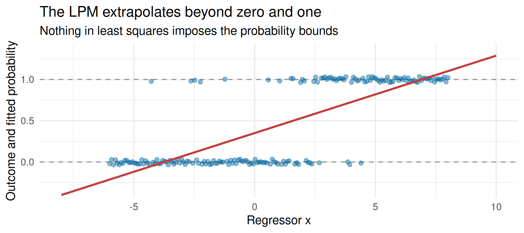
Within the observed middle range, a straight line can approximate a probability curve well. At sufficiently extreme \(x\), it must eventually cross zero or one.
Binary errors are heteroskedastic by construction
Write \(p_i=\Pr(y_i=1\mid x_i)\). Because a binary outcome is Bernoulli,
\[ \operatorname{Var}(y_i\mid x_i)=p_i(1-p_i). \]
The LPM error \(u_i=y_i-p_i\) therefore satisfies
\[ \operatorname{Var}(u_i\mid x_i)=p_i(1-p_i), \]
which changes with \(x_i\) whenever the probability changes with \(x_i\).
The practical consequence
The LPM needs heteroskedasticity-robust standard errors. Robust standard errors repair the inference; they do not repair out-of-range predictions or non-linearity.
The LPM trades shape for simplicity
What it buys. Coefficients are probability changes, estimation is fast, interactions remain straightforward, and high-dimensional fixed effects are easy to absorb.
What it costs. The conditional mean is forced to be linear, fitted probabilities can leave \([0,1]\), and the error is necessarily heteroskedastic.
The LPM is therefore not a failed logit model. It is a different approximation, often useful when the estimand is an average probability change rather than an individual prediction.
The next models impose the probability bounds directly.
From a line to an S-curve
A probability model needs a bounded map
A linear index \(x_i'\beta\) can take any real value. A probability cannot.
Logit and probit solve the mismatch by passing the index through a cumulative distribution function \(F\):
\[ \Pr(y_i=1\mid x_i)=F(x_i'\beta). \]
Every CDF is non-decreasing and maps the real line into \([0,1]\). A larger index can therefore raise the probability without ever pushing it outside its logical range.
Density and cumulative probability answer different questions
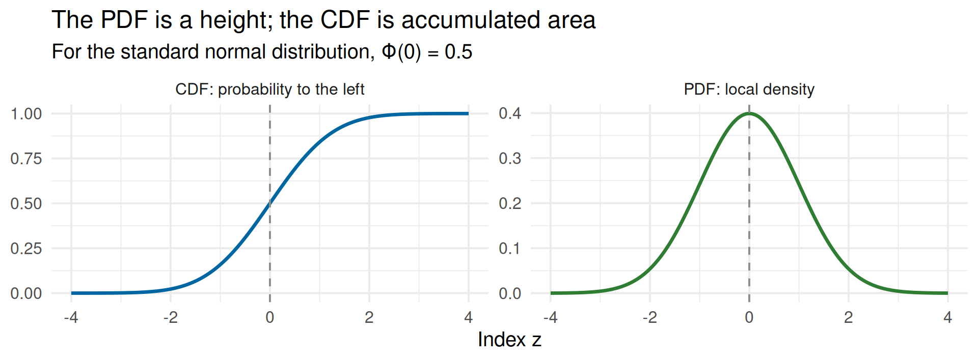
The CDF \(F(z)=\Pr(Z\le z)\) gives the probability accumulated up to \(z\). Its derivative \(f(z)=F'(z)\) is the PDF, which will determine how quickly a modelled probability changes.
A latent index turns a choice into a threshold
Imagine an unobserved continuous propensity
\[ y_i^*=x_i'\beta+\varepsilon_i. \]
We do not observe \(y_i^*\). We only observe whether it crosses zero:
\[ y_i= \begin{cases} 1 & \text{if } y_i^*>0,\\ 0 & \text{if } y_i^*\le 0. \end{cases} \]
The scale and units of \(y_i^*\) are arbitrary. Its role is to provide a coherent story for how a smooth probability produces a discrete outcome.
The error distribution determines the link
The threshold rule implies
\[ \begin{aligned} \Pr(y_i=1\mid x_i) &=\Pr(\varepsilon_i>-x_i'\beta\mid x_i)\\ &=1-F(-x_i'\beta) =F(x_i'\beta), \end{aligned} \]
where the last equality uses symmetry.
Two standard choices
Probit assumes a standard normal error and uses \(\Phi(x_i'\beta)\).
Logit assumes a standard logistic error and uses \(\Lambda(x_i'\beta)=1/(1+e^{-x_i'\beta})\).
Logit and probit differ mainly in the tails
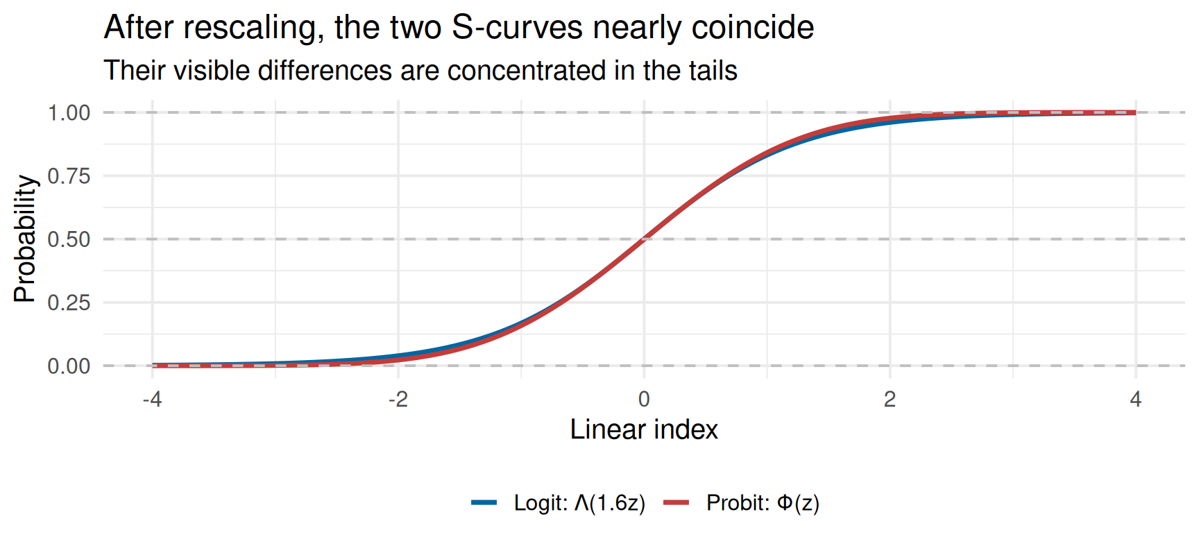
Raw logit coefficients are typically about 1.6 times raw probit coefficients because the latent scales differ. That numerical difference is not a substantive difference in probability effects.
The coefficient moves the index
In either model,
\[ p_i=F(x_i'\beta). \]
A one-unit increase in \(x_{ik}\) raises the index by \(\beta_k\). Its effect on probability is
\[ \frac{\partial p_i}{\partial x_{ik}} =f(x_i'\beta)\beta_k. \]
The same \(\beta_k\) creates a larger probability change near the steep middle of the S-curve than in either flat tail. There is therefore no single marginal effect unless we say where or over whom it is evaluated.
Non-linearity complicates fixed effects
In a linear probability model, unit fixed effects can be absorbed directly and every unit contributes to estimation.
Conditional fixed-effects logit avoids estimating thousands of unit intercepts by conditioning them out. That solution uses only units whose outcome switches over time; always-zero and always-one units contribute no identifying information.
Fixed-effects probit has no analogous conditioning trick and can suffer from the incidental-parameters problem when \(T\) is short. Random-effects logit and probit retain all units, but revive Lecture 5’s strong assumption that the unit effect is uncorrelated with the regressors.
Panel data do not choose the model for you
For many policy regressions, an LPM with unit fixed effects and clustered standard errors remains a transparent and defensible choice.
Maximum likelihood
OLS minimizes distance; MLE maximizes probability
OLS chooses coefficients that minimize a sum of squared residuals. That objective is convenient when the conditional mean is linear.
Logit and probit instead specify the full conditional probability of each binary outcome. Maximum likelihood chooses the parameter vector that makes the observed sequence of zeros and ones as probable as possible under that specification.
Maximum likelihood estimation
Given a statistical model and observed data, MLE finds the parameter values with the largest likelihood:
\[ \hat\beta_{\mathrm{MLE}}=\arg\max_\beta L(\beta\mid \text{data}). \]
A coin makes the likelihood visible
Suppose seven of ten independent flips are heads. If \(p\) is the probability of heads, the likelihood of that observed result is proportional to
\[ L(p)=p^7(1-p)^3. \]
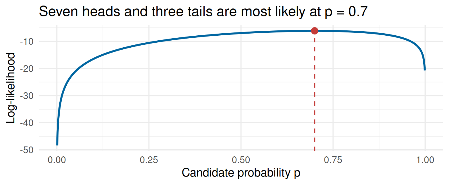
MLE formalizes the intuitive estimate \(\hat p=7/10\).
Each outcome contributes its modelled probability
Let \(p_i=F(x_i'\beta)\). One compact expression covers both possible outcomes:
\[ L_i(\beta)=p_i^{y_i}(1-p_i)^{1-y_i}. \]
When \(y_i=1\), the contribution is \(p_i\). When \(y_i=0\), it is \(1-p_i\).
Assuming observations are conditionally independent, the sample likelihood multiplies those contributions:
\[ L(\beta)=\prod_{i=1}^n [F(x_i'\beta)]^{y_i} [1-F(x_i'\beta)]^{1-y_i}. \]
Logs turn the product into a sum
Maximizing \(L(\beta)\) and maximizing \(\log L(\beta)\) give the same answer because the logarithm is increasing.
\[ \ell(\beta)= \sum_{i=1}^n \left[ y_i\log F(x_i'\beta) +(1-y_i)\log\{1-F(x_i'\beta)\} \right]. \]
Products of thousands of small probabilities are numerically fragile. The log-likelihood replaces multiplication with addition and is therefore easier for a computer to optimize.
Unlike the simple OLS formula, the first-order conditions generally have no closed-form solution. Software searches for the peak iteratively.
A successful optimization is not enough
MLE standard errors come from the curvature of the log-likelihood near its maximum. A sharp peak means the coefficients are precisely located; a flat peak means many values fit almost equally well.
Software should report that the optimizer converged. Failure to converge can signal poor scaling, near-perfect prediction, an overcomplicated specification, or a genuine identification problem.
Even after convergence, the usual causal warning remains. MLE estimates the specified conditional relationship; it does not make an endogenous regressor exogenous.
Interpreting non-linear models
Raw coefficients are not probability effects
| Model | Raw coefficient | Average probability change |
|---|---|---|
| Linear probability | 0.033 | 3.3 pp |
| Logit | 0.447 | 3.3 pp |
| Probit | 0.219 | 3.2 pp |
The raw logit and probit coefficients differ because the latent scales differ. The average changes in callback probability almost coincide.
Comparing raw coefficients across links, samples, or specifications can therefore be misleading. Translate them to the probability scale before communicating magnitude.
Marginal effects vary across observations
For a continuous regressor,
\[ ME_{ik} =\frac{\partial \Pr(y_i=1\mid x_i)}{\partial x_{ik}} =f(x_i'\hat\beta)\hat\beta_k. \]
The density \(f(\cdot)\) is largest near the centre of either S-curve. Two people can therefore share the same coefficient but have different marginal effects because their other covariates place them at different points on the curve.
The sign of the marginal effect follows the sign of \(\hat\beta_k\), but its size depends on the whole covariate vector.
A marginal effect at the mean describes a synthetic case
The marginal effect at the mean evaluates the derivative at \(\bar x\):
\[ MEM_k=f(\bar x'\hat\beta)\hat\beta_k. \]
It answers: what is the slope for a hypothetical observation whose every regressor equals its sample mean?
That case can be awkward. The mean person can simultaneously be 43% female, 27% in one occupation, and 18% in another. With interactions or strong non-linearity, the answer may poorly represent anyone in the sample.
MEM is easy to calculate, but its target should be stated explicitly.
The average marginal effect describes the sample
The average marginal effect first computes one derivative per observation, then averages:
\[ AME_k=\frac{1}{n}\sum_{i=1}^n f(x_i'\hat\beta)\hat\beta_k. \]
It answers: for the covariate distribution in this sample, what is the average local probability change associated with a one-unit increase in \(x_k\)?
The modern default
Report an AME when the goal is a sample-wide summary on the probability scale. State the population over which it is averaged.
A dummy needs a discrete change
The derivative formula treats a regressor as continuously variable. Race assignment in this experiment moves from zero to one, never by an infinitesimal amount.
For a binary regressor \(d\), use
\[ \Delta_i =F(x_i'\hat\beta\mid d_i=1) -F(x_i'\hat\beta\mid d_i=0), \qquad AME_d=\frac{1}{n}\sum_{i=1}^n\Delta_i. \]
This is what the callback table computed: predict every resume twice, change only the assigned name type, take the difference, and average.
Odds offer a second logit interpretation
For logit,
\[ \log\left(\frac{p_i}{1-p_i}\right)=x_i'\beta. \]
A one-unit increase in \(x_{ik}\) adds \(\beta_k\) to the log-odds and multiplies the odds by \(e^{\beta_k}\).
For the name indicator, the fitted odds ratio is 1.56. Holding sex and occupation fixed, the odds of a callback are about 56% higher for a white-sounding name.
Odds are not probabilities. When an event is rare they are close, but an odds ratio should never be described as a percentage-point change.
Our prediction, revisited
The LPM estimate is 3.3 percentage points. The logit and probit average discrete changes are 3.3 and 3.2 percentage points.
All three answers are almost identical because the fitted probabilities lie in a fairly narrow range and the race effect is summarized over the same resumes.
What the experiment identifies
Random assignment supports a causal interpretation of the name signal in this hiring context. It does not identify a universal effect of race in every labour market, nor the mechanism behind employers’ responses.
The model changes the functional form. The research design supplies the credibility.
Fit, testing, and prediction
Explanation and prediction ask different questions
For explanation, we care whether a regressor changes the outcome distribution and whether that change has a credible causal interpretation.
For prediction, we care how accurately fitted probabilities generalize to observations not used for estimation. A model can estimate an important average effect and still classify individuals poorly, especially when individual outcomes are noisy.
The resume experiment is exactly such a case: the treatment effect is clear, while callbacks remain rare and difficult to predict one by one.
The likelihood-ratio test compares nested models
Let \(\ell_U\) be the maximized log-likelihood of an unrestricted model and \(\ell_R\) that of a restricted model obtained by imposing \(q\) restrictions.
\[ LR=2(\ell_U-\ell_R) \overset{a}{\sim}\chi_q^2. \]
The statistic asks how much fit is lost when the restrictions are imposed. Testing all slopes jointly against an intercept-only model is the likelihood analogue of an overall \(F\)-test.
For our logit model, $LR=30.8 with 6 restrictions and \(p<.001\).
Pseudo-\(R^2\) is not variance explained
McFadden’s measure compares the full and intercept-only log-likelihoods:
\[ R^2_{\text{McFadden}} =1-\frac{\ell_{\text{full}}}{\ell_{\text{null}}}. \]
For our model it equals 0.011.
Despite the notation, this is not the fraction of outcome variance explained and should not be compared numerically with OLS \(R^2\). Its most useful role is comparing specifications fitted to the same outcome on the same sample.
A pseudo-\(R^2\) does not validate a causal interpretation and does not by itself measure out-of-sample performance.
Classification requires a threshold
A fitted logit produces probabilities, not zeros and ones. Classification adds a decision rule such as
\[ \hat y_i= \begin{cases} 1 & \text{if }\hat p_i>c,\\ 0 & \text{if }\hat p_i\le c. \end{cases} \]
The common threshold \(c=0.5\) is a convention, not a theorem. Lowering it identifies more actual positives but also creates more false positives.
The right threshold depends on the relative cost of the two mistakes. Disease screening, fraud detection, and marketing need not use the same cutoff.
A confusion matrix names the four outcomes
| Predicted 0 | Predicted 1 | |
|---|---|---|
| Actual 0 | True negative: 4478 | False positive: 0 |
| Actual 1 | False negative: 392 | True positive: 0 |
At the 0.5 threshold, the fitted model predicts no callbacks at all. Its accuracy is nevertheless 92.0%.
That apparently impressive number comes from the outcome imbalance, not useful discrimination between resumes.
Accuracy can reward an unhelpful model
A rule that always predicts the majority class is correct whenever the rare event does not occur. In our data, predicting “no callback” for every resume achieves 92.0% accuracy.
Sensitivity asks what fraction of actual positives were detected. Specificity asks what fraction of actual negatives were rejected. Precision asks what fraction of positive predictions were correct.
No single threshold-based metric captures the quality of the probability forecasts. Calibration, ROC curves, precision–recall curves, and proper scoring rules such as log loss add complementary information.
Never report accuracy without the baseline
For a rare event, always compare model accuracy with the majority-class rule and report metrics for the positive class.
Out-of-sample performance needs held-out data
Training-set fit rewards a model for explaining observations it has already seen. Prediction asks about genuinely unseen observations.
A clean evaluation separates training data from test data, estimates every model choice on the training set, and touches the test set only for the final comparison. With limited data, cross-validation repeats this separation across several folds.
Random splitting is inappropriate when nearby observations share information. Time-series prediction should respect time; clustered data should keep related observations together.
The estimand and the validation design must match the deployment setting.
Logit or probit is rarely the main decision
After translating to probabilities, logit and probit usually produce very similar answers. Logit offers the odds-ratio interpretation and is more common in many applied fields; probit follows directly from a normal latent-error model.
Choose a link for a substantive reason, a disciplinary convention, or comparability with earlier work. Then check whether conclusions are robust to the alternative.
Specification, identification, functional form, and the treatment of dependence usually matter more than choosing between these two S-curves.
Software
Estimate all three models with one changed line
Code
library(dplyr)
library(fixest)
library(haven)

resumes <- read_dta(
  "https://empirical-economics.netlify.app/tutorials/datafiles/lakisha_aer.dta"
) |>
  mutate(
    white = as.integer(race == "w"),
    female = as.integer(sex == "f"),
    occupation = factor(occupbroad)
  )

# LPM with heteroskedasticity-robust standard errors
lpm <- feols(
  call ~ white + female + i(occupation),
  data = resumes,
  vcov = "hetero"
)

# Logit and probit
logit <- glm(
  call ~ white + female + occupation,
  data = resumes,
  family = binomial("logit")
)
probit <- glm(
  call ~ white + female + occupation,
  data = resumes,
  family = binomial("probit")
)
Code
import pandas as pd
import pyfixest as pf
import statsmodels.formula.api as smf

resumes = pd.read_stata(
    "https://empirical-economics.netlify.app/tutorials/datafiles/lakisha_aer.dta"
)
resumes["white"] = (resumes["race"] == "w").astype(int)
resumes["female"] = (resumes["sex"] == "f").astype(int)
resumes["occupation"] = resumes["occupbroad"].astype("category")

lpm = pf.feols(
    "call ~ white + female + C(occupation)",
    data=resumes,
    vcov="hetero",
)
logit = smf.logit(
    "call ~ white + female + C(occupation)", data=resumes
).fit()
probit = smf.probit(
    "call ~ white + female + C(occupation)", data=resumes
).fit()
The link changes the scale of the raw coefficients. It should not change the definition of the outcome, sample, controls, or standard-error strategy.
Ask software for quantities on the probability scale
Code
Name the quantity in the output: raw coefficient, odds ratio, marginal effect at a specified case, average marginal effect, discrete change, or predicted probability.
Censoring and Tobit
A pile at zero is not necessarily binary
Annual hours worked, expenditure on a durable good, and research-and-development spending may all equal zero for many observations and take positive continuous values for the rest.
That outcome is not binary. The zeros and positive amounts both contain information about magnitude.
It is left-censored when an underlying continuous value exists below a known boundary but every value at or below that boundary is recorded as the boundary. A binary logit or probit would discard the differences among all positive observations.
Censoring and truncation remove information differently
With censoring, the observation remains in the sample, but its exact outcome beyond the boundary is hidden. We see a household with recorded expenditure zero, although its latent desired expenditure may be negative.
With truncation, observations beyond the boundary are absent from the sample entirely. A dataset containing only people with positive hours is truncated at zero.
Selection is different again: whether an outcome is observed depends on another process that need not be the outcome crossing a known boundary.
These mechanisms imply different likelihoods and should not be used as synonyms.
Tobit uses a censored latent outcome
For left-censoring at zero, Tobit assumes
\[ y_i^*=x_i'\beta+u_i, \qquad u_i\mid x_i\sim N(0,\sigma^2), \]
and the observation rule
\[ y_i=\max(0,y_i^*)= \begin{cases} 0 & \text{if }y_i^*\le 0,\\ y_i^* & \text{if }y_i^*>0. \end{cases} \]
One latent equation governs both crossing the boundary and the positive amount. That restriction is what makes Tobit more specific than merely “a model with zeros.”
OLS answers neither Tobit margin correctly
OLS on the positive observations conditions on \(y_i^*>0\). Selection then depends on the error, so
\[ E(u_i\mid y_i>0,x_i)\ne 0. \]
OLS on all observations treats the pile at zero as if it followed a linear conditional mean. Under Tobit, however,
\[ E(y_i\mid x_i) =\Phi(z_i)x_i'\beta+\sigma\phi(z_i), \qquad z_i=\frac{x_i'\beta}{\sigma}, \]
which is non-linear even though the latent outcome is linear.
The Tobit likelihood has two pieces
A censored observation contributes the probability of being at or below the boundary:
\[ \Pr(y_i^*\le 0\mid x_i)=\Phi\left(-\frac{x_i'\beta}{\sigma}\right). \]
A positive observation contributes the normal density at its observed value:
\[ \frac{1}{\sigma} \phi\left(\frac{y_i-x_i'\beta}{\sigma}\right). \]
MLE combines the probability mass at zero with the continuous density above zero. Dropping either piece discards information and changes the estimand.
Censoring bends the observed conditional mean
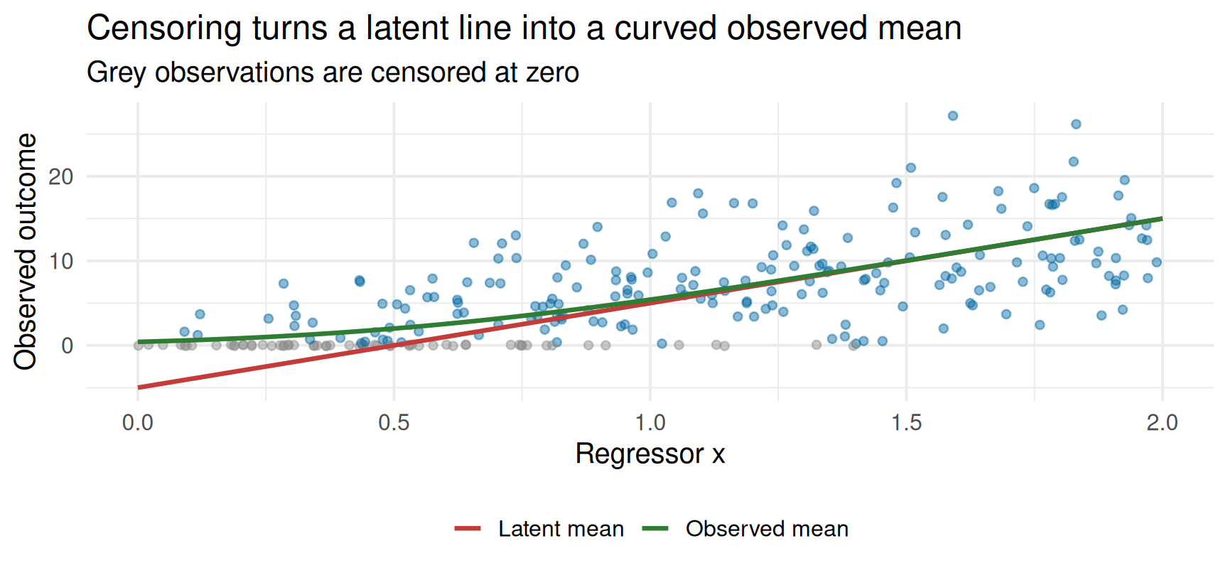
The line remains linear only for the unobserved \(y^*\). Censoring makes the mean of observed \(y\) flatten near the boundary.
A Tobit coefficient lives on the latent scale
The coefficient \(\beta_k\) is the effect of \(x_k\) on \(E(y_i^*\mid x_i)\), not directly on observed \(y_i\).
Three different effects may be substantively relevant:
\[ \begin{aligned} \frac{\partial \Pr(y_i>0\mid x_i)}{\partial x_{ik}} &=\frac{\beta_k}{\sigma}\phi(z_i),\\ \frac{\partial E(y_i\mid x_i)}{\partial x_{ik}} &=\beta_k\Phi(z_i). \end{aligned} \]
The first is an extensive-margin effect on crossing zero. The second combines that margin with the intensive margin, the amount observed when positive.
State which outcome you mean before reporting a marginal effect.
Tobit is a strong model, not a default for zeros
Standard Tobit assumes one normally distributed, homoskedastic latent equation determines both whether \(y\) is positive and how large it is.
That can be implausible. The factors that determine whether someone works may differ from those that determine hours conditional on working. A two-part or hurdle model allows those processes to differ.
Tobit is appropriate when censoring is the actual observation mechanism and its joint structure is defensible. A visible pile at zero is evidence of a data feature, not proof of the Tobit assumptions.
Takeaways
What did we learn?
- For a binary outcome, the conditional mean is the probability of success.
- The LPM estimates probability changes directly, but needs robust standard errors and can predict outside \([0,1]\).
- Logit and probit map a linear index through a CDF, which creates bounded S-shaped probabilities.
- MLE chooses parameters that maximize the modelled probability of the observed outcomes.
- A raw logit or probit coefficient moves a latent index; an AME summarizes movement on the probability scale.
- Discrete regressors require discrete probability comparisons, not derivatives.
- Accuracy depends on a threshold and can be deceptive for rare outcomes.
- Censoring preserves an observation at a boundary; truncation removes it from the sample.
- Tobit combines probability mass at the boundary with a density above it, and its coefficients describe a latent outcome.
Exit questions
Be able to answer these without looking back:
- Why is an LPM error heteroskedastic even when its conditional mean is correctly specified?
- What mathematical feature prevents logit and probit probabilities from leaving \([0,1]\)?
- What does observation \(i\) contribute to a binary likelihood when \(y_i=1\)? When \(y_i=0\)?
- Why can two observations have different logit marginal effects for the same regressor?
- Why is a derivative not the right effect for a zero–one regressor?
- How can a classifier be 92% accurate and still be useless?
- What is observed under censoring that is not observed under truncation?
- What does a Tobit coefficient describe directly?
Answers to the exit questions
- Binary variance. If \(p_i=\Pr(y_i=1\mid x_i)\), then \(\operatorname{Var}(u_i\mid x_i)=p_i(1-p_i)\). It changes with \(x_i\) whenever \(p_i\) does.
- The CDF. Both models set \(p_i=F(x_i'\beta)\), and every CDF maps the real line into \([0,1]\).
- Likelihood contribution. A success contributes \(p_i\); a failure contributes \(1-p_i\).
- Different locations. The effect is \(f(x_i'\beta)\beta_k\). Other covariates place observations on differently sloped parts of the S-curve.
Answers to the exit questions (continued)
- A discrete move. A dummy changes from zero to one. Predict at both values, subtract, and average if an AME is wanted.
- Rare outcomes. If only 8% are positive, always predicting zero is already 92% accurate while detecting none of the positives.
- The observation remains. Under censoring we see that an outcome is at the boundary; under truncation the entire observation is absent.
- The latent outcome. \(\beta_k\) directly shifts \(E(y_i^*\mid x_i)\). Effects on crossing the boundary or on observed \(y_i\) require transformation.
Looking ahead
Binary outcomes changed the functional form but not the central identification question: why is the regressor as good as randomly assigned after conditioning?
Lecture 7 turns that question into potential outcomes and asks how a comparison group can recover the missing counterfactual.
Appendix
The logit link and odds are equivalent
Starting from
\[ p_i=\frac{e^{x_i'\beta}}{1+e^{x_i'\beta}}, \]
we obtain
\[ 1-p_i=\frac{1}{1+e^{x_i'\beta}}, \qquad \frac{p_i}{1-p_i}=e^{x_i'\beta}, \qquad \log\left(\frac{p_i}{1-p_i}\right)=x_i'\beta. \]
This is why \(e^{\beta_k}\) is an odds ratio for a one-unit change in \(x_k\).
The PDF controls the steepness of the CDF
Because \(F'(z)=f(z)\),
\[ \frac{\partial F(x_i'\beta)}{\partial x_{ik}} =f(x_i'\beta)\beta_k. \]
For probit, \(f=\phi\) is the standard normal density. For logit,
\[ f(z)=\Lambda(z)\{1-\Lambda(z)\}=p_i(1-p_i). \]
The logit marginal effect can therefore be written as \(p_i(1-p_i)\beta_k\). It is largest at \(p_i=0.5\) and shrinks toward zero in both tails.
Source notes
- Bertrand, Marianne, and Sendhil Mullainathan (2004), “Are Emily and Greg More Employable Than Lakisha and Jamal? A Field Experiment on Labor Market Discrimination,” American Economic Review 94(4), 991–1013.
- Resume data are stored locally in
tutorials/datafiles/lakisha_aer.dta. - Binary-response and censored-regression material follows Wooldridge, Introductory Econometrics, Sections 7.5 and 17.1–17.2.
The End

Empirical Economics: Lecture 6 - Binary Outcome Data (Economics Track)