| Deal | Sun (\(X_S\)) | Rain (\(X_R\)) | Expected payoff | |
|---|---|---|---|---|
| 0 | Food truck | 5 | 0 | 2.5 |
| 1 | Canteen | 2 | 2 | 2.0 |
| 2 | Vending machine | 0 | 3 | 1.5 |
Pricing Lunch Discount Deals
No free lunch, but the discount deals are complimentary.
A two-state example that questions the meaning of value. NB! Since we are focused on valuing discount deals, the cost and value of the meals themselves don’t enter directly (if you pay close attention you might be able to spot the places where you can argue that they do indirectly).
Set-up I: Basics
Two equally likely states defines your day: sun (S) and rain (R). You buy exactly one lunch if you buy, but whether you buy is stochastic, i.e., on tough (rainy) mornings you are less likely to pack lunch and bring it from home.
- \(q_S = 0.25\): probability of buying lunch when sunny
- \(q_R = 0.75\): probability of buying lunch when it rains
Discount deals (payoffs \(X\)):
The university hands out discount deals for free, one per student, first come first served at a stand in the entrance hall.
Throughout, write \(a = 2\) for the canteen payoff (both states), \(b = 5\) for the food truck’s sunny payoff, and \(c = 3\) for the vending machine’s rainy payoff; the appendix leans on these letters.
Ranked by expected payoff, the food-truck deal is the clear winner and the vending deal the clear loser.
Valuation I: Timing
The value of a deal is its expected used payoff. Let m be the usage indicator (m = 1 if you buy lunch, 0 otherwise), so sun \(E[m | S] = q_S\) and rain \(E[m | R] = q_R\), and
Value = \(E[m X] = 1/2 (q_S X_S + q_R X_R)\).
| Deal | Expected payoff | Value | |
|---|---|---|---|
| 0 | Vending machine | 1.5 | 1.125 |
| 1 | Canteen | 2.0 | 1.000 |
| 2 | Food truck | 2.5 | 0.625 |
The value ordering is flipped compared to the expected-payoff ordering. Why? The big food truck discount is usually not needed (you more often bring your own lunch on sunny days), and while the vending deal only offers a moderate discount (pay-off), it pays exactly when you need it.
Your buying behavior acts as a Stochastic Discount Factor (SDF) determining the value (to you) of the discount since a discount is worthless in states where you don’t shop.
Conclusion: timing is covariance.
A bit of (standard) math makes this exact:
\[ E[mX] = E[m]\,E[X] + \operatorname{Cov}(m, X). \]
The first term is the deal’s expected pay-off scaled by a constant (the average SDF), which means that the ordering only depends on expected pay-off. The second term is what flipped the ordering above. Restating that Why? in slightly more formal language the food truck deal’s pay-off covaries negatively with your usage (it pays when you bring lunch anyway and don’t need it), whereas the vending deal’s pay-off covaries positively with your usage (it pays when you don’t bring lunch, i.e., exactly when you need it). Timing is this covariance. Average pay-off sets the first term, while timing of pay-offs sets the second, and here the second term is big enough to overturn the first.
| Deal | \(E[m]\,E[X]\) | \(\operatorname{Cov}(m, X)\) | Value \(E[mX]\) | |
|---|---|---|---|---|
| 0 | Vending machine | 0.75 | 0.375 | 1.125 |
| 1 | Canteen | 1.00 | 0.000 | 1.000 |
| 2 | Food truck | 1.25 | -0.625 | 0.625 |
Curious how each cell in this table is computed from the set-up’s parameters? See the appendix.
Set-up II: Appetite
It turns out that when we move from the simple world of lunch and the asset class of discount deals, we need to loosen two of our assumptions.
First a simple one: assets can be owned collectively and partially. In our example that means that you can get together with a group of friends and pool: everyone picks up their one free deal, the group throws all of them in a pot, and everyone shares the pay-offs equally, a portfolio of lunch deals. The deals themselves are still handed out whole, one per student, so a group of \(N\) friends pools exactly \(N\) whole deals, and your share of deal \(i\) is the number of copies your group picked up divided by the group size, \(\omega_i = n_i / N\). Two bookkeeping facts then come for free: the shares add up to one, and none of them can be negative, \[ \omega_T + \omega_C+\omega_V =1, \quad \text{and}\quad \omega_T, \omega_C,\omega_V \geq 0 . \]
Do we actually want to form portfolios in the current set-up? No. Value is linear in pay-offs, so the value of a portfolio is just the share-weighted average of the deals’ values: half canteen, half vending is worth \(\tfrac12 \cdot 1.0 + \tfrac12 \cdot 1.125 = 1.0625\), less than holding the vending deal alone (1.125). An average can never beat its best element, so a value maximizer puts everything on the single most valuable deal. If portfolios are ever to be worth forming, something else must be going on, which leads us to the second assumption, one we did not even state outright.
In the world outside lunch, the value of a euro is typically not zero or one. One might argue that even in the world of lunch, what a euro is worth to you depends on how many you already have. To make that precise, follow the euros to where they end up: consumption. A discount is money not spent on lunch, so the discount euros you collect are your daily budget for immediate self-care (fun money), and in a one-day world (student life?) there is nowhere else for them to go, so they are spent the day they arrive. Let \(C\) be the euro value of that day’s consumption, i.e., your portfolio’s pay-off when you buy lunch, and zero when you don’t.
How you spend those euros orders them. Picture your wants as a ladder of pleasures where the first euro gets spent on the thing you want most, the next on the second-best thing, and so on down the ladder.1 Euros are precious when \(C\) is small and less and less precious as the best wants get satisfied, so walking down the ladder gives a utility-of-consumption function \(u\) with the two properties that do all the work in this section: \[ u'(C) > 0 (\text{more is better}), \qquad u''(C) < 0 (\text{decreasing marginal value}). \]
We use the function whose ladder has the most regular rungs: constant proportional steps. Each extra euro of consumption multiplies the marginal value of the next one by the same factor, no matter how many you already hold. Formally, \[ u(C) = -e^{-\gamma C}, \] where the curvature constant \(\gamma\) sets how fast the ladder drops off. We pick \(\gamma = \ln(3/2) \approx 0.405\), so that the factor is exactly \(2/3\): every additional euro makes the next euro worth a third less.2
Notice that the weather still determines the likelihood of whether you buy lunch (\(q_S\) vs \(q_R\)), but the curvature decides what your consumption euros (fun or otherwise) are worth to you.
Valuation II: Risk
Pay-offs are still cash, but instead of caring about the expected realized discount you now care about the expected utility of the day’s consumption \(C\). Averaging over the weather and whether you buy, expected \(utility\) is
\[ \begin{align*} E[u(C)] &= \tfrac12\Big[q_S\, u(X_S) + (1-q_S)\, u(0)\Big] \\&\quad+ \tfrac12\Big[q_R\, u(X_R) + (1-q_R)\, u(0)\Big]. \end{align*} \tag{1}\]
The no-buy terms \(u(0)\) are the same for every holding, so they never decide a portfolio choice.
To compare holdings in euros rather than in units of utility (what is that even?), we translate each holding into its certainty equivalent (CE). The sure daily consumption that would make you indifferent between that and the risky consumption \(C\) the holding delivers. This is defined as the number that solves \[ u(CE) = E\big[u(C)\big], \]
so that a holding and its certainty equivalent sit at the same height on the utility ladder. And because consumption is nothing but the deal’s pay-off, the certainty equivalent lives on the same euro scale as every table above and compares to them directly. For how the CARA \(CE\) is computed see the appendix.
The best mix visualized:
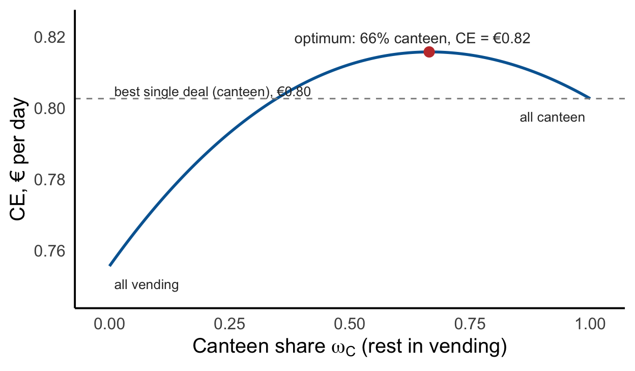
The best holding is the portfolio 66% canteen, 34% vending, and no food truck at all, worth a sure €0.82 a day against €0.80 for the best single deal (canteen). The optimum needs a group of just \(N = 3\): two friends who grabbed canteen deals and one who grabbed a vending deal. In numbers:
| Holding | Sun (\(X_S\)) | Rain (\(X_R\)) | \(CE\) | |
|---|---|---|---|---|
| 0 | Optimal portfolio | 1.33 | 2.34 | 0.816 |
| 1 | Canteen only | 2.00 | 2.00 | 0.803 |
| 2 | Vending machine only | 0.00 | 3.00 | 0.756 |
| 3 | Food truck only | 5.00 | 0.00 | 0.283 |
The curvature made the smooth (weather safe) option of the canteen more valuable and made a portfolio the winner.
For more on the food truck deal’s zero weight, see the appendix.
Conclusion: risk is non-smooth (volatile) pay-offs
Diversification pays because \(u\) curves. Smoothing pay-off across states is better than loading it on one state, even at the same expected pay-off (Jensen’s inequality). The linear criterion of Section I does not care about that risk (an average never beats its best element). Portfolios only start to matter once the euro-ladder enters. What did not change is that good and bad states are still labelled by usage, the food truck is still shunned because its generosity still arrives at the wrong time, and next, we’ll turn to what \(E[m X]\) look like when your stochastic discouunt factor is not just whether a euro matters but also how much.
What happened to Value and the SDF?
The certainty equivalent sounds a lot like a measure of value (and it is) but it doesn’t look at all like \(E[mX]\). It is important at this point to specify what kind of value \(E[mX]\) is: it is marginal value, the value of one just a bit more of an asset, given what you already hold. In Section I that qualifier was invisible, because value was linear, so every little bit was worth the same and holdings were irrelevant, which is exactly why portfolios were pointless there. With curvature the more you hold, the less the next little bit is worth (walking down the euro-consumption-ladder).
A marginal value also has a second name. It is your willingness to pay (a reservation value). TThe daily rate at which you would want neither a bit more nor a bit less of the asset, given what you already have. Deliberately, we do not call it a price even though the two have a bunch of things in common (a difference is a market and we’ll get back to that below in Set-up III).
Notice that nothing about marginal value depends on what you are currently holing. Any holding comes with its own marginal values. So let us take an arbitrary portfolio and derive its marginal value. The pay-off you actually collect is the product of two random variables, the pay-off when you buy lunch \[ X^P = \omega_C X^C + \omega_T X^T + \omega_V X^V \] and whether you buy or not \(\mathbb{I}_{\text{buy}}\) which is either 0 or 1 with state-dependent probabilities \(q_S\) and \(q_R\) (our old SDF).
Our indifference condition says that if we could own a little bit more or less of the portfolio at the daily rate \(v\) we should not want to. Your deals were free, so think of the hypothetical extra bit as a subscription you could take out: \(v\) is its daily rate, a rate you agreed on in advance, but pay on the day, out of the day’s cash.3 Let’s give that hypothetical “amount of portfolio minus rate” that we want more or less than what we already have, the symbol \(\psi\). Your willingness to pay is then whatever rate \(v\) makes you choose \(\psi = 0\): at that rate, trading nothing is exactly what you want. We can now write the little bit more or less as a derivative of our expected utility of the consumption funded by the portfolio minus rate, i.e., \(C^P = \mathbb{I}_{\text{buy}}X^P + \psi (\mathbb{I}_{\text{buy}}X^P -v)\), with respect to the hypothetical scale \(\psi\) and demand that it equals zero at \(\psi = 0\). It is useful to look back at the expected utility of consumption formula (Equation 1) and notice that the expectation is just a probability weighted sum4, so we can just as well differentiate the sum as we can sum the derivatives. Formally, \[ \begin{align} 0&=\frac{\partial E[u(C^P)]}{\partial \psi} = E\left[u'(C^P)\frac{\partial C^P}{\partial \psi}\right] = E\left[u'(C^P)(\mathbb{I}_{\text{buy}}X^P - v)\right] \\&\iff E\left[u'(C^P)\mathbb{I}_{\text{buy}}X^P\right] = E\left[u'(C^P)v\right], \end{align} \] and since the daily rate was agreed on in advance, \(v\) is the same number in every state and can be pulled out of the expectation, so we finally have \[ E\left[ \frac{u'(C^P)}{E\left[u'(C^P)\right]}\mathbb{I}_{\text{buy}}X^P \right] = v. \] Wow, look at that, \(E[mX]\) is back, with \[ m = \mathbb{I}_{\text{buy}}\frac{u'(C^P)}{E\left[u'(C^P)\right]} = \mathbb{I}_{\text{buy}} \frac{u'(\mathbb{I}_{\text{buy}}X^P )}{E\left[u'(\mathbb{I}_{\text{buy}}X^P)\right]} \] where we use that \(\psi=0\). The stochastic discount factor is now personal twice over: it still asks whether a euro matters in a state (the usage indicator, Section I’s \(m\)) and now also how much it matters there (marginal utility of consumption). And through \(C^P\) that second part depends on what you hold: different holdings, different SDF, different marginal values.
So where, in all of this, is optimality? Nowhere yet, and that is worth dwelling on: marginal values exist at every holding. Optimality is about what the marginal values tell you to do.
Suppose you held only the canteen deal, Section I’s most valuable single deal, so a perfectly reasonable grab at the stand. Your marginal value for the vending deal would be €0.69, against €0.62 for the canteen itself: at the margin the vending deal is worth more to you, so swapping a slice of canteen for a slice of vending at any rate in between makes you better off. A holding whose marginal values disagree comes with a profitable trade attached, and the optimal portfolio (our two-thirds canteen, one-third vending, no truck) is exactly the holding at which the profitable trades run out. The promise of the stochastic discount factor is not just to value one asset, but any asset on the menu, so below are your marginal values at the optimum for all four assets considered above, but before you look:
TipPredict first
One of the four assets is valued differently from the other three. Which one is it? Is its marginal value higher or lower than the rest?
| Asset | Sun (\(X_S\)) | Rain (\(X_R\)) | Marginal value \(v = E[mX]\) | |
|---|---|---|---|---|
| 0 | Canteen | 2.00 | 2.00 | 0.608 |
| 1 | Vending machine | 0.00 | 3.00 | 0.608 |
| 2 | Optimal portfolio | 1.33 | 2.33 | 0.608 |
| 3 | Food truck | 5.00 | 0.00 | 0.507 |
If Section I’s ranking made you bet on the vending deal standing out at the top, this table is the productive surprise: at your optimum there is no ranking left. The indifference condition that defined \(v\) is exactly the statement that everything you hold is worth the same at the margin: had the canteen and vending deals carried different marginal values, you could have shifted a little weight from the low-value deal to the high-value one and been better off, contradicting that your portfolio was optimal. The portfolio itself matches because it is just a bundle of the other two. And the food truck is the exception that proves the rule: its marginal value sits strictly below the common level, which is the inequality version of the very same condition, and precisely why its weight is zero. Section I ranked the deals; optimizing traded the ranking away.
Interlude: trading without prices
Before any market opens, the two value concepts we now own (certainty equivalents for holdings, marginal values for slices) already answer every “would you trade?” question. Stay with the eater holding only the canteen deal.
Whole deals. Would you swap your canteen deal for a vending deal, one for one? Swapping whole deals is a question about holdings, and two holdings compare by their certainty equivalents: the canteen deal is worth a sure €0.80 a day, a vending deal only €0.76, so you refuse, even though the table above your prediction callout showed the vending deal carrying the higher marginal value at your holding. There is no contradiction: the marginal value prices the first slice, and slices get less valuable as they pile up. Matching your canteen deal takes 1.11 vending deals. And the food truck? No number of truck deals — none — matches the canteen deal: truck deals pay only on sunny days, extra sun-day euros land on ever-flatter rungs of the ladder, and the certainty equivalent of an all-truck holding saturates at €0.33 no matter how many you stack. Rain-day euros simply cannot be bought with sun-day euros here.
Pools. The friend pool from Set-up II is a whole-deal trade too (a swap of deal slices at the fixed rate one-for-one), and the CE ledger shows who signs up. In the three-friend pool (canteen, canteen, vending), everyone gains: each canteen-grabber’s certainty equivalent rises by €0.013 a day and the vending-grabber’s by €0.060. But try pooling a canteen-grabber with a truck-grabber: the pool sits at half-canteen half-truck, the truck-grabber would gain €0.33 a day, and the canteen-grabber would lose €0.19, so the pool never forms. Gains from trade exist between these two (the truck-grabber gains far more than the canteen-grabber loses), but a pool that trades everything one-for-one cannot deliver them. Unlocking that surplus needs a side payment: a price.
Rents. So put a number on it. Suppose the canteen-holder could rent a vending deal: keep their canteen deal, receive the vending pay-offs on top, and pay a fixed daily rate for it. The most they would pay is the rate at which they are indifferent (their reservation rent), and under the constant-steps ladder it is simply the certainty-equivalent difference between the two holdings: €0.44 per day for a whole vending deal on top of the canteen deal. This exactness is the pay-off of choosing CARA: rents and certainty equivalents live on the same euro ruler, so “what would you pay?” never needs more than a CE subtraction.5 For a thin slice the same logic hands back the marginal value \(v\) from the previous section: reservation rents are CE differences, and marginal values are their per-slice limit.
Set-up III: Scarcity
So far every trade was voluntary and bilateral, and nothing forced anyone to hold anything. One more dose of realism changes that. The university printed a fixed batch of deals (the print run) and handed out all of them, first come first served. Once the stand is empty the swap option is gone: whatever mix the print run contained is now, deal by deal, in somebody’s pocket. Collectively, the students must hold the print run. That is the situation real investors are in (the shares of every company exist in fixed supply and every one of them is always in someone’s portfolio), and it is the missing ingredient that turns marginal values into prices.
To let students rearrange who holds what, open a secondary market: students trade deal shares with each other, and trades settle on the same clock as the deals pay: a daily rate, agreed when you trade, paid every day out of your fun money, so rent and pay-off land in the same day’s cash. Renting a share to a classmate means receiving its daily rate; renting one from them means paying it. (On a day your deals pay nothing, paying a rent means consuming less of something else: lunch money, say. Under the constant-steps ladder it never matters which rung of your wider life a euro comes from, so the bookkeeping is harmless.) Note the rates themselves are new: the deals were handed out free and carry no fees; what gets priced here is the trade, never the handout.
Valuation III: Price
What daily rates clear this market? The logic is the mirror image of Section II. There, the rates were fixed (one-for-one at the stand) and your holdings moved until marginal values agreed with the rates. Now the holdings are fixed in aggregate (the print run must be held), so the rates must move until everyone is content to hold it. Prices are whatever makes the marginal values true: the clearing price of each deal is its marginal value \(v\) evaluated at the print-run portfolio, and the letter \(p\) finally earns its name, \[ p = E[mX]. \]
One more CARA convenience makes “evaluated at the print-run portfolio” unambiguous: because risk appetite does not depend on wealth, every student, whatever they grabbed at the stand, wants exactly the same risky position at the market’s prices, namely their per-capita share of the print run. Everyone ends up holding the market; the only thing your grab at the stand decides is which side of the rent payments you are on.6
TipPredict first
The university printed equal numbers of all three deals. Use Sections I and II to guess: which deal commands the highest price, and does any ranking come back at all?
| Deal | Print run = optimal mix | Equal print run | Truck-heavy print run | |
|---|---|---|---|---|
| 0 | Canteen | 0.608 | 0.647 | 0.689 |
| 1 | Food truck | 0.507 | 0.328 | 0.243 |
| 2 | Vending machine | 0.608 | 0.774 | 0.888 |
Three print runs, three price columns, one lesson each:
- Print run = optimal mix. If the university happened to print exactly the mix Section II’s eater wants (67% canteen, 33% vending, no truck), the market clears at Section II’s own marginal-value table: held deals at the common level, truck below. The equalization was not an artifact of the quota economy; it is what prices look like when supply matches desire.
- Equal print run. With the truck genuinely in the batch, somebody must hold it, and no ranking-free equilibrium exists: prices spread out, and the ordering that comes back (vending €0.77 above canteen €0.65 above truck €0.33) is Section I’s value ordering, reborn as a price ordering. Section II traded the ranking away only because it was free to walk away from the truck; a market that must absorb the print run cannot.
- Truck-heavy print run. Print more trucks and the truck price falls further (€0.51 → €0.33 → €0.24 as the truck’s share of the print run goes \(0 \to \tfrac13 \to \tfrac12\)). The least-desired deal must still be held by someone, so its price falls until holding it stops hurting. Scarcity (and its opposite) is priced.
And the first-come-first-served scramble? It has become a wealth lottery. At the equal print run, the deal in your pocket is your endowment, and the market prices it: a vending grabber holds €0.77-a-day of value, a truck grabber only €0.33. Everyone then rents their way to the same market portfolio: the truck grabber pays a net €0.26 a day for the upgrade, funded by the canteen and vending grabbers’ net receipts of €0.06 and €0.19, so the lottery’s sting is not what you end up holding (everyone holds the market) but what you pay to hold it. Notice, finally, who never appears in this story: the university set no prices, and neither did anyone else. Prices came out of preferences meeting a fixed supply, which is exactly the half of asset pricing that Sections I and II, with their free quota and movable holdings, could not reach.
Appendix
A bit of additional math for those who can’t get enough
We can calculate the unconditional \(E[m]\) from it’s conditional value and the probability of each state (weather) which is just \(Pr(S)=Pr(R) = 1/2\) and therefore \[ E[m] = Pr(S) E[m|S] + Pr(R) E[m|R] = 1/2(q_S + q_R) = 0.5. \]
The covariance term is just as computable. Notice that since there are only two possible kinds of weather we have \(Pr(R)=1-Pr(S)\). Furthermore, since the weather is the only variation linking the SDF and the pay-off, both are (up to constants) scalings of the same Bernoulli variable, we could call it the sun indicator, so their covariance is the product of the indicator’s variance, \(Pr(S)(1-Pr(S))=\tfrac14\), and two differences between the states. For the stochastic discount factor which actual varies across two dimensions: weather and probability of buying lunch; the weather dimension is the relevant part (it covaries wiht pay-offs), which means the difference we need is \(E[m|S]-E[m|R] = q_S - q_R\). Putting the elements together, \[ \begin{aligned} \operatorname{Cov}(m, X) &= Pr(S)\big(1-Pr(S)\big)\,\big(E[m|S]-E[m|R]\big)\,(X_S-X_R) \\ &= \tfrac{1}{4}\,(q_S - q_R)\,(X_S - X_R) \\ &= -0.125\,(X_S-X_R). \end{aligned} \] Since \(\tfrac{1}{4}\,(q_S - q_R) =-0.125 < 0\), everything about a deal’s timing is in the sign of \((X_S - X_R)\). Any deal paying more in sun than in rain covaries negatively with usage (food truck: \(-0.125\,(5 - 0) = -0.625\)), any deal paying more in rain covaries positively (vending: \(-0.125\,(0 - 3) = 0.375\)), and a state-independent payoff covaries with nothing (canteen: \(X_S = X_R\) gives exactly \(0\)), matching the decomposition table in Valuation I.
More additional math for whom it may concern: the Section II SDF factorizes
Written out in full, expected utility over the whole day is
\[ E[u] = \sum_{s \in \{S,R\}} Pr(s)\Big[\, q_s\, u\big(\omega \cdot X_s\big) + (1-q_s)\, u(0) \,\Big]. \]
The no-buy terms \((1-q_s)u(0)\) do not involve the portfolio \(\omega\), so they drop out of any comparison between holdings, leaving the criterion used in Section II: \(\sum_s Pr(s)\, q_s\, u(\omega \cdot X_s)\), which is exactly \(E[m\, u(C)]\) with \(m\) the usage indicator from Section I.
Now ask what one extra slice of a deal is worth. Differentiating with respect to that deal’s share gives its marginal value,
\[ E\big[\, m \cdot u'(C) \cdot X \,\big], \]
so Section II prices pay-offs with the SDF \(m \cdot u'(C)\): the Section I part answers whether a euro matters in a state, the new part answers how much. Two consequences:
- Section I is the small-holdings limit. At \(\omega = 0\), consumption is zero in every state, so \(u'(0)\) is a common constant and the SDF is proportional to plain \(m\): the first slice of any deal is valued exactly as Section I says. Curvature only bites as holdings grow.
- The optimum in closed form. With the food truck excluded, the first-order condition between the canteen and vending shares reads \(2 q_S\, e^{-\gamma C_S} = q_R\, e^{-\gamma C_R}\), i.e. \[ C_R - C_S = \frac{\ln\!\big(q_R / (2 q_S)\big)}{\gamma} = \frac{\ln(3/2)}{\ln(3/2)} = 1: \] hold the mix that puts rain-day consumption exactly €1 above sun-day consumption. Since the gap along the canteen–vending edge is \(c(1-\omega_C)\), this gives \(\omega_C = 1 - \tfrac13 = \tfrac23\), exactly where the numerical search behind the figure lands. The truck stays excluded because its marginal value at the optimum, 0.507, is below the (equalized) marginal values of the canteen and vending deals, both 0.608; shifting any weight into the truck lowers expected utility. (It sits at exactly \(\tfrac56\) of the common level: the truck replicates from the held deals as \(\tfrac52 C - \tfrac53 V\), a bundle whose shares net to \(\tfrac56\) of one quota unit.)
The certainty equivalent, computed. With \(u = -e^{-\gamma C}\), the defining equation \(u(CE) = E[u(C)]\) inverts to
\[ CE = -\frac{1}{\gamma}\, \ln\!\Big( E\big[e^{-\gamma C}\big] \Big), \]
an exponentially tilted average of the day’s possible consumption levels: \(X_S\) with weight \(\tfrac12 q_S\), \(X_R\) with weight \(\tfrac12 q_R\), and zero with the remaining no-buy probability.
Why a base budget would have changed nothing, the one-line proof promised in Set-up II. Hand the eater any sure background amount \(B\) on top, so the day’s consumption levels become \(B+X_S\), \(B+X_R\), and \(B\). Then \(e^{-\gamma B}\) factors out of the tilted average and the \(\ln\) turns it into “\(+B\)”: the certainty equivalent shifts one-for-one with the budget, and every comparison between holdings (the optimum, all marginal values, every trade below) is untouched. Deleting the budget was free. (A CARA-only privilege: under a ladder that flattens with wealth, like \(\log\), the budget is load-bearing.)
Jensen’s inequality puts any concave-\(u\) certainty equivalent below the arithmetic average of consumption, which is exactly \(E[mX]\), Section I’s value. So
\[ CE \;\le\; E[mX]: \]
the deal’s certainty equivalent is Section I’s value minus a risk charge, and shrinking that charge is precisely what the diversified portfolio does. (Even the safe canteen pays a small charge: the day’s consumption still varies with whether you buy at all, and that buy-or-not variation is one no holding on this menu can smooth away.)
Why zero truck, and an identity
The truck’s zero, verified. Fix any food-truck share \(\omega_T\), split the rest between canteen and vending as cleverly as possible, and record the best certainty equivalent you can reach. That frontier falls the moment \(\omega_T\) leaves zero and keeps falling all the way down (the computation behind the figure checks strict decrease at every grid point):
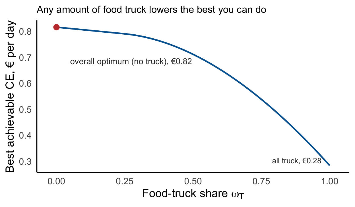
Note what this is and is not: it is a fact about this eater. The truck is the only deal that can push pay-off toward the sunny state, so an eater whose buying were concentrated in sun would hold it; ours buys in the rain, so every reallocation away from the truck helps. Nothing dominates the truck state-by-state.
The identity. The canteen enjoys stronger protection. Could a mix of truck and vending replace it (pay at least \(a\) in both states)? A mix with truck share \(\omega\) pays \(\omega b\) in sun and \((1-\omega)c\) in rain, so replacement needs \(\omega \ge a/b\) and \(\omega \le 1 - a/c\) at once: possible if and only if \(\tfrac{a}{b} + \tfrac{a}{c} \le 1\), i.e. \(a(b+c) \le bc\). The canteen is un-substitutable precisely when
\[ a(b+c) > bc. \]
Now expand the sharp threshold that Section I’s value-inversion required (checked numerically for the parameters used here): \(a^2 > (b-a)(c-a) = a^2 + bc - ab - ac\), which simplifies to \(ab + ac > bc\): the same inequality. The parameter pattern that lets the safe deal win on value in Section I is exactly the pattern that makes it impossible to synthesize from the risky deals in Section II. One condition, two jobs: it powers the timing inversion, and it guards the safe deal’s seat in the portfolio.
Returns and risk premia
The equalized marginal values invite the obvious objection (real assets have different prices!), and Set-up III delivered on it; the remaining reconciliation runs through returns. It sits here in the appendix rather than in the main text: the main argument has done its job once \(p = E[mX]\) lands, and this is where a course in asset pricing takes over.
Real assets differ in price because shares are arbitrary units with different pay-offs. Per euro invested every asset costs the same (€1), and the equalization reappears as the most famous equation in asset pricing: \(E[mR_i] = 1\) for every asset \(i\), with \(R_i\) the pay-off per euro. From there it is two lines to risk premia. Applied to the risk-free asset, \(E[m]R_f = 1\) gives \(R_f = 1/E[m]\); applied to any asset via the same covariance decomposition as Section I’s “timing is covariance”, \[ 1 = E[m]\,E[R_i] + \operatorname{Cov}(m, R_i) \;\;\Longrightarrow\;\; E[R_i] - R_f = -R_f\,\operatorname{Cov}(m, R_i). \] Risk premia are covariance with the SDF and nothing else: an asset’s own variance never appears. It is Section I’s lesson restated per euro invested: what flipped values there is what creates premia here.
Bookkeeping note: to price a risk-free asset (pays €1 whether or not you buy lunch) the usage indicator must sit on the pay-off side, not inside the SDF (the same expectation regrouped, \(m = u'(C)/E[u'(C)]\) pricing used pay-offs \(\mathbb{I}X\)). Then \(E[m] = 1\), so \(R_f = 1\) exactly (the main text’s subscription footnote made precise: the daily rate is paid the same day, so the risk-free rate is zero by construction) and the premium collapses to \(E[R_i] - 1 = -\operatorname{Cov}(m, R_i)\).
Why \(R_f = 1\) is exact here and nowhere else: the model has informational timing (the price is agreed before the weather reveals itself) but no consumption timing; price and pay-off settle out of the same day’s cash, so there is no separate “today” marginal utility and no role for impatience. In the standard two-date version, \(m = \beta\, u'(c_{t+1})/u'(c_t)\), and \(R_f = u'(c_t) \big/ \beta E[u'(c_{t+1})] \neq 1\) in general: impatience (\(\beta < 1\)) and expected consumption growth both push the risk-free rate up. Adding that second date would move \(E[m]\), and nothing else; the premium equation above survives verbatim. That is Cochrane’s clean separation: the level of \(E[m]\) prices time, the covariance with \(m\) prices risk. The one-day design zeroes out the time price on purpose so that covariance is the only thing left standing: “timing is covariance” is about state timing, not calendar timing. (The subscription framing carries exactly these two requirements: the daily rate is one number across states because it was agreed in advance, and no time passes between paying and collecting because it is paid on the day.)
In this economy, with \(E[R_i]\) = Section I value / marginal value at the optimum:
| Asset | \(E[R]\) | Risk premium | |
|---|---|---|---|
| 0 | Vending machine | 1.850 | 0.850 |
| 1 | Optimal portfolio | 1.713 | 0.713 |
| 2 | Canteen | 1.645 | 0.645 |
| 3 | Food truck | 1.234 | 0.234 |
All premia are positive: every deal pays only in buy states, where consumption is positive and euros matter less than average. And the ordering is Section I’s roles inverted. Vending, Section I’s hero, now carries the highest premium and the shunned truck the lowest, because the optimal portfolio loaded rain with pay-off, rain is the consumption-rich state at the optimum, so the vending deal pays exactly where euros are cheapest (it has become the risky, procyclical asset) while the truck pays into the relatively consumption-poor sunny buy-state, the closest thing to a hedge on the menu. Equal marginal values, unequal expected pay-offs: vending’s fatter expected pay-off per euro is its compensation for paying into a state your own holdings made rich. You keep buying the valuable deal until it becomes the risky one, and the premium is where that process stops. (This is also the germ of every factor model: CAPM and friends are parameterizations of what \(m\) covaries with.)
Further reading: Price
In general, an SDF is a random variable that can seem almost magical, as it makes the fundamental relationship \(p = E[mX]\) between price \(p\) and pay-off \(X\) true. Set-up III showed the mechanics for one market; two structural facts sit behind it. If a market has no arbitrage, no way to buy a pay-off cheap and sell it dear at a sure profit, then some (positive) SDF pricing everything traded is guaranteed to exist. If the market is furthermore complete, enough traded pay-offs to span every state (in our case two buy-states, so at least two deals that pay differently across them), that \(m\) is unique and we go from an SDF to the SDF.
And note which half of the economy each of our set-ups nailed down. Set-ups I and II were a quota economy: every deal counted one unit against your handout quota, so the exchange rates between deals were fixed (one-for-one at the stand) and quantities did all the adjusting, which is why marginal values, not prices, came out the other end. Set-up III flipped it: quantities were fixed (the print run must be held) and the rates did the adjusting. These are the two poles of a general-equilibrium chicken-and-egg (endowment economies where supply is fixed and prices adjust, versus linear technologies where the price is pinned at production cost and quantities adjust), and real economies sit in between, with an upward-sloping supply curve moving both at once. The genuinely exogenous things retreat one layer back, to preferences, technology, and endowments. This discussion, these questions, and the equation above are the backbone of John Cochrane’s book Asset Pricing (2005), and his Asset Pricing course notes and recorded lecture videos hosted on his own site, johnhcochrane.com.
Footnotes
The same ladder runs a firm. Its euros go into the best investment project first, then the next-best, and diminishing returns make the value of funds concave. That forms the basis of the production-side twin of the consumption asset pricing model we are working towards here. The firm’s first-order condition prices assets the way the consumer does here (production-based asset pricing, or investment CAPM).↩︎
This constant-steps family is called CARA (constant absolute risk aversion), the workhorse of a lot of models of trade. It does not have so-called wealth effects, which means that for a CARA consumer, being richer never changes the appetite for risk. The classic contrast are utility functions that exhibit CRRA (constant relative risk aversion), the simplest version is log-utility.↩︎
Two design choices hide in that sentence. Agreed in advance makes \(v\) the same number in every state. Paid on the day means the rate and the pay-off settle out of the same day’s cash: no time passes between paying and collecting, so the model values risk while deliberately switching off intertemporal valuation (impatience, interest rates). That other half of asset pricing needs a second date; we gave it the day off.↩︎
With finitely many states an expectation is literally a probability-weighted sum. With infinitely many possible states (a Normally distributed pay-off, say), the weighted sum becomes an integral against the probability distribution, but the same move still works: differentiating under an integral is fine under mild regularity conditions, so nothing that follows would change.↩︎
Exact for CARA only. Under a ladder whose steps flatten as you get richer (log, say), paying a sure rent makes you effectively poorer and more risk-averse, and the true reservation rent falls short of the CE difference, a wealth effect.↩︎
This “everyone holds the market” logic, suitably dressed up, is the germ of two-fund separation and the CAPM. Here it is exact because preferences are identical CARA; heterogeneity would spread holdings out without changing the pricing logic.↩︎