library(data.table)

base_url <- "https://empirical-economics.netlify.app/tutorials/datafiles/"
ff5  <- fread(paste0(base_url, "F-F_Research_Data_5_Factors_2x3.csv"), skip = 3)
mom  <- fread(paste0(base_url, "F-F_Momentum_Factor.csv"), skip = 13)
ff25 <- fread(paste0(base_url, "25_Portfolios_5x5.csv"), skip = 15)Betting Against Beta: From Flat SML to Traded Factor
Data companion for Lecture 8’s asset-pricing application (Finance track)
How to use this document
This is the pricing half of Lecture 8’s asset-pricing application: once returns-data-companion.qmd has built a genuine monthly return, what does the profession actually do with it? The case study is Betting Against Beta (Frazzini and Pedersen 2014) — a flat security market line, a leverage-constraint story for why it is flat, a tradable factor built on that story, and four different tools (a time-series regression, a TED-spread mechanism test, Fama-MacBeth vs. Giglio-Xiu, and IPCA) turned on the same question from different angles.
Three source-license tiers coexist in this one document, so each code chunk is marked plainly. Ken French’s factor library, the JKP low-beta factor (jkpfactors.com, CC BY-NC 4.0 — Jensen, Kelly & Pedersen 2023, full citation in Sources), the TED spread (FRED), and the Pastor-Stambaugh liquidity series are free and committed to data/: the benchmark-world setup (French loading, excess returns, the 5×5 sanity grid, an FF5 feols regression), the JKP three-versions CAPM-alpha wedge, and the JKP leg of the TED-mechanism regression run live, eval: true, in front of you. Everything built on licensed Compustat (the own-BAB construction, the daily-beta rebuild and size screen, the entire IPCA lens) or on AQR’s redistribution-restricted BAB series (AQR’s own TED regressions, the premium-cost figure, the FM-vs-GX/GXZ calibration and TED-innovations grid, which are also Python-backed and compute-heavy) is shown eval: false: exact, runnable code, with every number quoted from a ledger built by actually running it once, provenance kept in the private working notes. Two figures matter for the same reason: figures/bab_own_sml.png is git-tracked (a derived image from licensed Compustat is fine by this repo’s convention); figures/bab_premium_cost_aqr.png is not (AQR’s terms block even derived images), so that exhibit is described and quoted rather than shown.
Two sibling companions bracket this one. returns-data-companion.qmd builds the monthly return panel this document prices; daily-returns-companion.qmd covers the deep daily-cleaning machinery (BCWX’s decimal-error correction and eight-filter survivor chain) that the daily-beta rebuild below depends on, including a re-derive of this document’s own numbers on the fully cleaned panel — cross-referenced where it matters. One data caveat recurs throughout: TED (FRED’s TEDRATE) was discontinued at the source in January 2022 (the LIBOR phase-out), so every TED exhibit below — live or quoted — runs on the fixed window 1986-01..2022-01; it is flagged again at first use in each section rather than assumed.
Standing up the benchmark world
The rest of this document’s application needs test assets and factors to run GX against later. This part is entirely free data: the Ken French Data Library. This opening loads the 25 size/BM portfolios, the standard FF93 test-asset panel, plus the FF5 factors and momentum, and points at GX-202 for the real, big-cross-section GX application later in the lecture. We do not rebuild GX-202 here, only its ingredients.
Loading the test assets and factors
library(data.table)

ff5  <- fread("data/ff5_factors.csv")
setnames(ff5, 1, "date")
ff5[, date := as.IDate(date)]

mom  <- fread("data/momentum_factor_umd.csv")
setnames(mom, 1, "date")
mom[, date := as.IDate(date)]

ff25 <- fread("data/25_sizeBM_25.csv")
setnames(ff25, 1, "date")
ff25[, date := as.IDate(date)]
Building excess returns
Subtract the risk-free rate from every portfolio column at once, extended to the FF5 set (adds RMW, profitability, and CMA, investment, to Mkt-RF/SMB/HML) plus momentum as a sixth series for the liquidity fork’s BAB comparison later:
# Joins align on month; RF is NA before FF5's 1963-07 start, so the
# excess-return panel is effectively FF5-era even though mom reaches 1927.
merged <- ff25[ff5, on = "date"][mom, on = "date"]
port_cols <- setdiff(names(ff25), c("date", "year"))

excess <- merged[, ..port_cols][, lapply(.SD, function(x) x - merged$RF)]
excess[, date := merged$date]What a factor model claims (and does not)
A time-series regression of a test asset’s excess return on the FF5 factors
\[ R_{it} - R_{ft} = \alpha_i + b_i \, MKT_t + s_i \, SMB_t + h_i \, HML_t + r_i \, RMW_t + c_i \, CMA_t + \epsilon_{it} \]
is exactly the machinery Lecture 7’s GRS test operates on: a joint test that \(\alpha_i = 0\) for every test asset, run on the traded-factor world, where every right-hand-side object is itself a return you could go buy. See the lecture 7 material for the full GRS treatment; this opening does not re-teach it.
What this machinery cannot do is price a candidate that is not itself a traded return: a macro state variable, a sentiment index, a funding-cost spread. GRS needs every right-hand-side object to be a return. That is the gap the Giglio-Xiu three-pass estimator closes, and why the fork below exists: to hand GX three genuinely non-traded (or not cleanly traded) candidates once this benchmark world is standing.
library(fixest)

m <- feols(I(`SMALL HiBM` - RF) ~ `Mkt-RF` + SMB + HML + RMW + CMA, data = merged)
summary(m)
OLS estimation, Dep. Var.: I(`SMALL HiBM` - RF)
Observations: 756
Standard-errors: IID
Estimate Std. Error t value Pr(>|t|)
(Intercept) 0.150447 0.072664 2.070460 3.8751e-02 *
`Mkt-RF` 0.962703 0.017579 54.765710 < 2.2e-16 ***
SMB 1.082294 0.025439 42.544611 < 2.2e-16 ***
HML 0.411511 0.032821 12.538083 < 2.2e-16 ***
RMW -0.003963 0.033688 -0.117647 9.0638e-01
CMA 0.243732 0.048991 4.975076 8.0932e-07 ***
---
Signif. codes: 0 '***' 0.001 '**' 0.01 '*' 0.05 '.' 0.1 ' ' 1
RMSE: 1.91835 Adj. R2: 0.905452The application: the case of the backwards portfolio
The mystery, opened cold
The most successful investor in history holds a portfolio of boring stocks — ones that swing noticeably less than the market, reliably so. The professionals explicitly paid to beat him — mutual funds — systematically hold the exciting ones. The person with the best track record alive does the opposite of the people trying to catch him. Why?
Put numbers on it (Frazzini and Pedersen 2014, holdings tests): Berkshire Hathaway’s ex ante portfolio beta is 0.90–0.91, significantly below one (t up to −3.65); the value-weighted mutual-fund sector sits at 1.08, significantly above one (t = 2.16). Neither is an accident of one year; both are stable features of decades of holdings data. Keep the word “beta” out of the classroom version of this opening — “swings less than the market” is the whole concept needed, and the measurement instrument arrives in the next section as a tool of the investigation, not a definition.
Is the crime real? The flat SML, again
Lecture 7 already put the security market line on screen and found it too flat: the BJS-style decile exhibit gave \(\hat\mu_0 = 4.3\) and \(\hat\mu^M = 3.6\) annualized against the market’s own \(7.2\). Lecture 8 opens the file lecture 7 left on the table. Two upgrades turn that exhibit from an anomaly into a category fact:
- It is everywhere. Frazzini-Pedersen find the same relative flatness in 18 of 19 international equity markets (Austria the lone, insignificant exception), in Treasuries across maturity, in corporate bonds by rating — where the far high-beta end turns the line over entirely (Distressed tranche alpha −1.11%/mo, t = −5.47) — and in futures.
- It is in our own data. The return panel
returns-data-companion.qmdconstructs is enough to reproduce it: rolling 60-month pre-formation betas (plain OLS — a stated simplification of FP’s correlation/volatility-split estimator), ten value-weighted beta deciles, 1979–2010. Realized decile betas run 0.52 to 1.85, cleanly monotone; the fitted cross-sectional line is \(0.375 + 0.189\,\beta\) %/mo against the CAPM-predicted slope of 0.581 (the market’s own mean excess return) — a third of the predicted slope, with the CAPM alphas declining from D1 to D10. The BJS picture, on a panel every student here can rebuild.
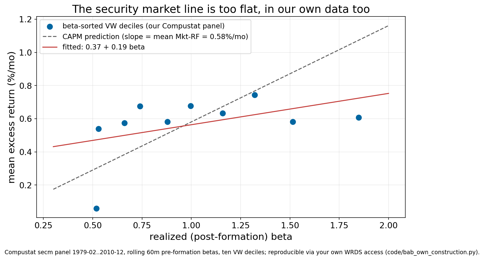
(Static, git-tracked figure: a derived image from licensed Compustat is fine by this repo’s convention. Backing code: the own-BAB construction script (E-B1) and the SML figure script; numbers outputs/bab-numbers-b1.md.)
The culprit: a constraint, not a mistake
Fisher Black proposed the mechanism in 1972, the same year the anomaly was first documented; Frazzini-Pedersen formalized and tested it four decades later. Investors who cannot lever — by regulation, charter, or plain unwillingness — but who want more expected return have exactly one route: tilt into high-beta assets. Their demand bids high-beta assets up and leaves low-beta assets cheap. Capturing that cheapness at market risk requires leverage — precisely the resource the constrained majority lacks. The friction creates the mispricing and blocks its own correction.
Frazzini and Pedersen state the finding, and its reach across markets, in their own words:
“All real-world investors face funding constraints such as leverage constraints and margin requirements, and these constraints influence investors’ required returns across securities and over time. We find empirically that portfolios of high-beta assets have lower alphas and Sharpe ratios than portfolios of low-beta assets. The security market line is not only flatter than predicted by the standard CAPM for US equities (as reported by Black, Jensen, and Scholes (1972)), but we also find this relative flatness in 18 of 19 international equity markets, in Treasury markets, for corporate bonds sorted by maturity and by rating, and in futures markets. We show how this deviation from the standard CAPM can be captured using betting against beta factors, which could also be useful as control variables in future research (Proposition 2). The return of the BAB factor rivals those of all the standard asset pricing factors (e.g., value, momentum, and size) in terms of economic magnitude, statistical significance, and robustness across time periods, subsamples of stocks, and global asset classes.”
The equilibrium version (FP Proposition 1) is one board equation:
\[ E(r_i) - r_f = \psi_t\,(1-\beta_i) + \beta_i \cdot \text{MRP}, \]
where \(\psi_t\) is the wealth-weighted average Lagrange multiplier on the funding constraint — how tight leverage is economy-wide. The live sign check: \(\psi_t = 0\) collapses to textbook CAPM; \(\psi_t > 0\) raises the intercept and flattens the slope, making alpha positive below \(\beta = 1\) and negative above. The friction is not a vibe; it is a parameter with a predicted sign, and the rest of this section chases that sign through three different kinds of evidence.
The strategy: turning a flat line into a return series
Betting Against Beta is the flat SML made tradable: go long low-beta assets, short high-beta assets, and rescale both legs to a beta of one at formation, so the market-risk term cancels and what remains is compensation for the constraint. On US equities 1926–2012 the factor earns 0.70% per month (t = 7.12), a CAPM alpha of 0.73% (t = 7.44), a four-factor alpha of 0.55% (t = 5.59), and an annualized Sharpe ratio of 0.78 — rivaling value and momentum on their own turf.
Three versions of this factor appear in this course’s material, and the differences are part of the lesson.
AQR’s published series (quoted)
The paper-faithful construction (rank-weighted legs, each rescaled to beta one). Redistribution is prohibited by AQR’s terms of use, so this companion quotes computed numbers with provenance and ships the refetch script rather than the data. Our re-run on the FP window (1930-12..2012-03, T = 976) reproduces the paper’s cells: mean 0.68%/mo, CAPM alpha 0.73 (t = 6.9), four-factor alpha 0.54, Sharpe 0.70. On the modern FF5 era (1963–2026) the FF5+UMD alpha is 0.30%/mo (Newey-West t = 2.1): the premium survives the modern factor zoo, at less than half its historical alpha (outputs/bab-numbers-b4.md).
The JKP factor-zoo version — seen live
The betabab_1260d factor (jkpfactors.com, CC BY-NC 4.0) uses the same beta measure as the paper (the correlation/volatility split), but the zoo’s standardized construction: capped-value-weighted terciles, without the beta-one leg rescaling. The consequence is dramatic and exactly on-message — and because the series is free, committed data (data/jkp_betabab_usa_monthly.csv), it is the one version of this three-way comparison this companion can run in front of you rather than only report.
library(data.table)
library(fixest)

jkp <- fread("data/jkp_betabab_usa_monthly.csv", skip = "date,ret")
jkp[, date    := as.IDate(date)]
jkp[, ym      := format(date, "%Y-%m")]
jkp[, ret_pct := ret * 100]                       # decimal monthly return -> %/mo

ff3 <- fread("data/ff3_factors.csv")
setnames(ff3, 1, "date")
ff3[, date := as.IDate(date)]
ff3[, ym   := format(date, "%Y-%m")]

# JKP dates are month-end, French dates are month-start: merge on year-month,
# not the raw date (the convention used throughout this companion's R code).
dt <- merge(jkp[, .(ym, ret_pct)], ff3[, .(ym, mktrf = `Mkt-RF`)], by = "ym")
setorder(dt, ym)
dt[, t  := .I]
dt[, id := 1L]                                    # dummy panel unit for fixest's NW() vcov

c(raw_mean_pct = mean(dt$ret_pct), n_months = nrow(dt))
raw_mean_pct n_months
-0.08322538 1169.00000000 m_capm <- feols(ret_pct ~ mktrf, data = dt, panel.id = ~id + t)
summary(m_capm, vcov = NW(6))OLS estimation, Dep. Var.: ret_pct
Observations: 1,169
Standard-errors: Newey-West (L=6)
Estimate Std. Error t value Pr(>|t|)
(Intercept) 0.470588 0.109155 4.31117 1.7608e-05 ***
mktrf -0.826039 0.056694 -14.57002 < 2.2e-16 ***
---
Signif. codes: 0 '***' 0.001 '**' 0.01 '*' 0.05 '.' 0.1 ' ' 1
RMSE: 3.4007 Adj. R2: 0.62657Over 1928–2025 the raw mean printed above is small — on the wrong side of a “low-risk premium” to look impressive by itself — while the CAPM alpha below it is large and highly significant. A supervisor-verified rerun of exactly this regression recorded α ≈ 0.49%/mo (t ≈ 4.4) and β ≈ −0.84 (outputs/bab-numbers.md, “E-B2” verdict); the live output above should land in the same neighborhood. The mechanism is arithmetic, not a puzzle: the unrescaled long-low/short-high portfolio carries a net market beta of about −0.84, and the market premium it forgoes swamps the alpha in the raw mean (\(\alpha + \beta\,\overline{MktRF}\) reproduces the raw mean to the fourth decimal in the ledger’s recomputation). The zoo version drops the leverage feature that embodies the mechanism, and the raw mean shows it: a factor’s name is not its construction. (Correlation with the AQR series over their common window: 0.53. Source, license, and construction caveat in outputs/bab-numbers-b2.md.)
Our own version (quoted)
From the panel returns-data-companion.qmd builds. The honest form is the unlevered low-minus-high decile spread: it correlates at 0.75 with the JKP factor (it is the same kind of object) and 0.44 with AQR’s, and it reproduces the raw-mean-vs-alpha wedge live in our own data — net market beta −1.33, raw mean −0.55%/mo, CAPM alpha +0.22%/mo (insignificant on our 32-year window; stated as such). The levered paper construction is where a monthly-beta panel gives out: rescaling each leg by \(1/\beta\) requires betas that never sit near zero, and rolling monthly OLS betas — even with FP’s own shrinkage toward one (\(w = 0.6\), their Eq. 15) — are too noisy for it (our attempt produced ex-ante low-leg betas as small as 0.003, and dividing by that is not a portfolio). FP estimate betas from daily data precisely for this reason, and doing exactly that (the next section) turns the failed monthly exercise into a working factor. The leverage feature is the one part of BAB you cannot improvise on monthly data, and discovering that by trying is what motivates the daily rebuild (outputs/bab-numbers-b1.md has the monthly-beta post-mortem; outputs/bab-numbers-b9.md the daily resolution).
Building it properly: daily betas, and the universe you keep
The monthly-beta dead end has a clean exit: estimate betas the way Frazzini and Pedersen do, from daily returns. Pulling Compustat’s daily file (comp.secd, 63 million firm-days, 1984–2010) and forming pre-formation betas the FP way, one-year daily-return correlations with the market and longer rolling volatilities with their shrinkage toward one, resolves the pathology that killed the monthly version. The ex ante low-leg beta now bottoms out at 0.45, and not one of 264 formation months has a low-leg beta below 0.2, where the monthly estimator had produced betas as small as 0.003. The \(1/\beta\) leg rescaling that was impossible on noisy monthly betas is routine on daily ones. Daily and monthly beta rankings still correlate at 0.63: the same firms, ranked more reliably.
With the leverage feature restored, our own BAB-proper on 1989–2010 earns 2.22% per month (t = 8.1, annualized Sharpe 1.73) and correlates 0.83 with AQR’s published series over that window, three times AQR’s own 0.78% on the same months. That gap is not a triumph; it is a warning, and chasing it down is the whole payoff of building the factor yourself. The excess comes from the smallest stocks. Drop the bottom market-capitalization quintile at formation and the premium collapses to 0.558% per month (t = 2.1, Sharpe 0.46), while the correlation with AQR rises to 0.94 (a median-cap cut gives 0.46 and 0.87 for the two screens). Three-quarters of the unscreened premium lived in bottom-quintile Compustat micro-caps, where illiquidity, bid-ask bounce, and missing delisting returns (see daily-returns-companion.qmd) manufacture paper profits no tradable portfolio could capture. AQR screens those names out; our first pass did not, and the factor looked spectacular for exactly the wrong reason.
Important
The quotable own-BAB number is the screened 0.558%/mo; the unscreened 2.22 is the labelled micro-cap contrast, kept visible because the contrast is the lesson. Read the universe before you read the Sharpe ratio, and note the construction only validates (ρ = 0.94 with AQR) once that universe is honest.
NoteRobustness check: does the full BCWX daily-cleaning chain change this?
The two numbers above are built on daily betas that pass only two price-only cleaning screens plus a ret > 10 null — not the full eight-filter, decimal-error-corrected chain daily-returns-companion.qmd builds (its # Does it matter downstream? The FP beta re-derive section). Re-running the identical construction on the fully BCWX/JKP-screened daily panel gives a clean answer to “does this matter”: the size-screened headline is robust — 0.558%/mo (t = 2.14, corr. AQR 0.944) moves only to 0.571%/mo (t = 2.20, corr. AQR 0.934), essentially unchanged. The unscreened number is not robust at all: 2.22 collapses to 0.87%/mo (t = 3.41), while its correlation with AQR rises from 0.83 to 0.95. That collapse sharpens, rather than overturns, the micro-cap lesson: roughly three-fifths of the naive 2.22 (the drop from 2.22 to 0.87%/mo is 60.7%) was contaminated daily betas from unscreened micro-cap and decimal-error returns, stacked on top of the portfolio-level over-weighting the size screen already fixes — two compounding problems, both fixable, converging on the same clean, AQR-matching destination. (outputs/bab-numbers-b9-bcwx.md.)
(Numbers: outputs/bab-numbers-b9.md; the daily pull, cleaning screens, and FP-beta estimator are written up as a lesson in daily-returns-companion.qmd and the daily BAB pipeline script.)
The funding-tightness mechanism, as a coefficient
The mechanism regression makes the picture a coefficient: BAB returns on the TED spread (3-month LIBOR minus 3-month T-bill), the standard funding-tightness proxy, in level and in change. Frazzini-Pedersen’s US-equity estimates load negatively on the contemporaneous change in TED — exactly the model’s Eq. (11): tightening funding forces deleveraging by the arbitrageurs holding the low-beta trade, and BAB loses money now. The lagged level also enters negatively (−0.025, t = −5.24, to −0.038, t = −4.78, depending on controls) — which FP flag candidly as the opposite of what a literal reading of TED-as-\(\psi_t\) predicts for future expected returns (Eq. 12).1 That candor is worth a paragraph in class: a clean theoretical prediction meets the messy job of proxying a latent equilibrium object, and the authors say so instead of burying it.
TED window flag: every TED exhibit below, like every one above, runs on 1986-01..2022-01 (data/ted_spread_monthly.csv, FRED TEDRATE) — the series was discontinued at the source in January 2022 (LIBOR phase-out).
AQR: the headline cell (quoted)
Our own run of the regression (AQR BAB, 1986-02..2022-01, N = 432, Newey-West 12 lags — the TED-mechanism regression script) reproduces both facts on three decades of data FP did not have: the contemporaneous ΔTED coefficient is −5.0% per month per percentage point of TED (t = −3.8) — a one-point funding spike costs the strategy about five percent that month — and the lagged level enters at −1.7 (t ≈ −3.3), FP’s anomalous sign again (in FP’s decimal-return units our joint-spec level coefficient is −0.024, inside their published −0.025..−0.038 range). Dropping 2008–09 entirely barely moves it: the mechanism is not one crisis. (outputs/bab-numbers-b5.md, gates B5.1/B5.2 — this leg needs AQR’s redistribution-restricted series, so it is quoted rather than run.)
JKP: the renderable cell — seen live
On the JKP tercile version a market control is not optional (its construction is not beta-neutral like AQR’s, so mktrf has to absorb the residual market exposure directly) — and because JKP, TED, and FF5 are all free, committed data, this is the one leg of the TED mechanism the ledger itself calls “the renderable cell” (outputs/bab-numbers-b5.md), and the one this companion can run rather than only quote:
library(data.table)
library(fixest)

ted <- fread("data/ted_spread_monthly.csv")
setnames(ted, c("date", "TEDRATE"), c("date", "ted_pp"))
ted[, date := as.IDate(date)]
ted[, ym   := format(date, "%Y-%m")]
setorder(ted, date)
ted[, ted_lag1 := shift(ted_pp, 1)]
ted[, dted     := ted_pp - ted_lag1]

ff5 <- fread("data/ff5_factors.csv")
setnames(ff5, 1, "date")
ff5[, date := as.IDate(date)]
ff5[, ym   := format(date, "%Y-%m")]

jkp <- fread("data/jkp_betabab_usa_monthly.csv", skip = "date,ret")
jkp[, date    := as.IDate(date)]
jkp[, ym      := format(date, "%Y-%m")]
jkp[, ret_pct := ret * 100]                       # decimal -> %/mo

dt_jkp <- merge(ted[, .(ym, ted_lag1, dted)], jkp[, .(ym, ret_pct)], by = "ym")
dt_jkp <- merge(dt_jkp, ff5[, .(ym, mktrf = `Mkt-RF`)], by = "ym")
setorder(dt_jkp, ym)
dt_jkp <- dt_jkp[ym >= "1986-02" & ym <= "2022-01"]   # TED window, see above
dt_jkp[, t  := .I]
dt_jkp[, id := 1L]                                    # dummy panel unit for fixest's NW() vcov

# The mandatory-market-control spec (the ledger's "B5.4" gate):
m_jkp_dted  <- feols(ret_pct ~ dted + mktrf,            data = dt_jkp, panel.id = ~id + t)
# The joint level-and-change spec, for comparison against the AQR cell above:
m_jkp_joint <- feols(ret_pct ~ ted_lag1 + dted + mktrf, data = dt_jkp, panel.id = ~id + t)

summary(m_jkp_dted, vcov = NW(12))
OLS estimation, Dep. Var.: ret_pct
Observations: 432
Standard-errors: Newey-West (L=12)
Estimate Std. Error t value Pr(>|t|)
(Intercept) 0.618474 0.189441 3.26473 0.001183 **
dted -1.302896 1.263394 -1.03127 0.302994
mktrf -0.813108 0.079563 -10.21968 < 2.2e-16 ***
---
Signif. codes: 0 '***' 0.001 '**' 0.01 '*' 0.05 '.' 0.1 ' ' 1
RMSE: 3.46257 Adj. R2: 0.51793summary(m_jkp_joint, vcov = NW(12))OLS estimation, Dep. Var.: ret_pct
Observations: 432
Standard-errors: Newey-West (L=12)
Estimate Std. Error t value Pr(>|t|)
(Intercept) 1.044255 0.288714 3.61692 0.00033343 ***
ted_lag1 -0.773368 0.419110 -1.84526 0.06568530 .
dted -1.726168 1.302477 -1.32530 0.18577483
mktrf -0.820492 0.080097 -10.24367 < 2.2e-16 ***
---
Signif. codes: 0 '***' 0.001 '**' 0.01 '*' 0.05 '.' 0.1 ' ' 1
RMSE: 3.44853 Adj. R2: 0.520714The first regression above is the ledger’s designated B5.4 gate. A supervisor-recorded run of this exact specification found ΔTED = −1.30 (Newey-West-12 t ≈ −1.0), against the gate’s own pass condition “ΔTED coefficient < 0” — passed, but only on sign: the ΔTED sign FP predict survives, the significance does not. The joint specification (second summary) adds the lagged level and typically drags the ΔTED t-statistic slightly further from zero in magnitude terms while remaining insignificant; both are shown because the AQR cell above is reported as the joint specification, and comparing like with like matters. The unrescaled zoo factor is a noisier probe of the funding channel — one more consequence of dropping the leg-rescaling that is JKP’s departure from FP’s actual construction.
Our own unlevered spread: no signature (quoted)
Our own unlevered decile spread (market control, 1986–2010) shows no TED signature at all (ΔTED t = 0.3) — consistent with the channel living in the leverage implementation itself, though on that shorter window it is equally consistent with noise; both readings stand. (outputs/bab-numbers.md, gate E-B5.3.)
Pricing the friction itself: FM vs GX on a non-traded candidate
BAB is a traded return, so lecture 7’s time-series machinery prices it directly. The friction is not traded: nobody sells you a \(\psi_t\). If funding tightness is a state variable investors pay to hedge, its risk price must be estimated from the cross-section — and that is exactly the estimation problem where lecture 7’s Fama-MacBeth two-pass and the Giglio-Xiu three-pass part ways. Omitted priced factors bias the two-pass twice — in the time-series betas and again in the cross-sectional regression; GX’s answer is to project the candidate on the panel’s principal components first. One candidate, both estimators, same test assets: the cleanest possible view of what the three-pass buys.
NoteEverything in this section is quoted, not run
Both estimators here are Python-backed (the GX three-pass, the Fama-MacBeth two-pass, the GXZ/SPCA variant) and the bootstrap bands underneath them are compute-heavy — 1000-draw resamples at every cell, across a full grid of candidates and panels. Every number below is quoted from the ledger cell named next to it; nothing in this section executes when the document renders.
First, grade the estimators where the truth is checkable. BAB is traded, so its premium needs no estimator at all: the sample mean is the answer (0.766%/mo on 1963–2024, NW t = 4.5, on GX-202’s window). Running both estimators anyway, on the identical window and panel, is the calibration step (the traded-vs-FM/GX calibration script, all in %/mo of BAB):
| λ̂ | vs the own mean of 0.766 | |
|---|---|---|
| Fama-MacBeth two-pass | 1.006 (t = 3.9) | overshoots by ~30% |
| GXZ/SPCA (supervised) | 0.565 [0.34, 0.74] | undershoots less; truth near the band’s edge |
| GX three-pass, restricted | 0.538 [0.35, 0.67] | undershoots; band excludes the truth |
| GX three-pass, free | 0.433 [0.23, 0.58] | undershoots; band excludes the truth |
All the estimators miss a premium we can see, and the misses are informative. GX’s shortfall is spanning, in two distinct layers. The panel is not missing the right assets: it contains French’s 25 size-beta portfolios, which alone span half of BAB. The first layer is PC-truncation — BAB is not a leading-PC direction of this panel (a “weak factor” in PCA’s sense despite being strongly priced), so the seven components GX keeps carry only 45% of it, climbing to 72% only by the hundredth component. The supervised GXZ estimator exists for exactly this layer, and behaves as designed: screening on correlation with the candidate first, it reaches 63% spanning with the same seven components and moves λ̂ from 0.43 toward 0.57. The second layer no estimator can cross: regressing BAB on all 202 portfolios tops out at 81%, because BAB’s time-varying rank weights and beta-one leg rescaling are a dynamic strategy that no static combination of portfolios replicates. FM’s overshoot is the two-pass’s own pathology on betas that proxy for more than the named factor; on the modern subwindow its intercept is \(\hat\gamma_0 = 0.66\)%/mo, Black’s zero-beta-rate excess sitting inside the estimator that is supposed to measure the premium. Hold these failure modes in hand before reading the next table.
The candidate: TED innovations (expanding-window AR(2) purge on lagged information only, mirroring the discipline used for the news study below; usable 1991-03..2022-01, T = 371; TED window flag as above). The panels: the GX-202 French block and this course’s own 204-portfolio Compustat panel — the latter also large enough to run the supervised (GXZ/SPCA) variant built for weak factors, which matters because a funding variable has no reason to be a strong factor in an all-equity panel.
The verdict the data returns (pre-registered as acceptable): a genuine null, with the estimator gap in plain view. All premia in %/mo per 1-sd of the candidate (\(\tilde p = 7\); full grid with \(\check p \in
\{7,10,13\}\), both \(\gamma_0\) cells, and bootstrap bands in outputs/bab-numbers-b6.md):
| estimator | panel | \(\hat\lambda_g\) (free) | (restricted) | excl. 0? |
|---|---|---|---|---|
| GX three-pass | GX-202 (T=371) | −0.020 | −0.028 | no |
| GX three-pass | wide N=204 (T=238) | −0.012 | −0.021 | no |
| GXZ/SPCA | wide N=204 | −0.045 | — | no |
| GX three-pass | combined N=406 | −0.021 | −0.033 | no |
| Fama-MacBeth | GX-202 | −0.236 (t = −1.41) | Shanken t −1.37 | no |
| Fama-MacBeth | wide N=204 | −0.085 (t = −0.43) | no |
Three readings, in order of importance:
- Every cell has the sign the constraint story predicts — an asset that pays off when funding tightens is a hedge, so its risk price should be negative — and no cell can tell that sign from zero. The measured-cells sentence: the equity cross-section 1991–2022, at the spans we can actually build, does not deliver a detectable funding-liquidity premium under any of the three estimators. The calibration above says how much weight “detectable” carries: on this same panel the estimators recover a strongly-priced traded factor at only 56–74% of its true premium (GXZ at the top of that range), so a similarly weakly-spanned funding candidate could carry a premium of this table’s order and still print as zero. The null is genuine; it is a statement about the panel’s reach as much as about the candidate.
- FM and GX disagree by an order of magnitude on identical data (−0.236 vs −0.028 on GX-202, the same standardized candidate). On a null candidate the data cannot adjudicate which is closer to the truth — which is precisely the OVB lesson: the estimator choice is not a detail, and the two-pass’s exposure to omitted-factor and errors-in-variables bias is why the gap can be this large.
- The GXZ loadings gate reads CONCENTRATED (16 of 204 portfolios carry the candidate’s exposure), so the supervised estimator had real screening leverage and still found nothing — the same stronger-null logic the news study below leans on. The raw-ΔTED robustness cell (T = 432, back to
- is no different (−0.027/−0.044, bands straddle).
Three labelled contrasts frame the result:
- Funding vs market liquidity. Pastor-Stambaugh innovations — the course’s running non-traded example — measure market liquidity (price impact of trading); TED measures funding liquidity (the arbitrageur’s cost of leverage). Acharya-Pedersen (2005) is the bridge if one is needed. The two are cousins, not twins, and the same-window PS cell makes that concrete: on 1991–2022 PS liquidity prices at +0.084 free / +0.246 restricted — also null on this window, against its own significant full-window restricted cell (+0.362 on 1976–2010). The funding candidate does not inherit PS’s power, and window choice matters as much as candidate choice.
- Exposure is not spanning: BAB and traded illiquidity. A cleaner, complementary question about the same two liquidities: not “does a non-traded liquidity state variable carry a risk price” (the GX question above), but “does BAB’s own alpha survive once a traded liquidity factor sits on the right-hand side.” The answer is a clean exposure-without-spanning. BAB loads significantly and positively on a CRSP-free traded illiquidity factor built from our own panel (Amihud, illiquid-minus- liquid quintiles, pre-formation: \(\beta = 0.22\)–\(0.32\), \(t = 2.2\)–\(4.7\)) — BAB’s micro-cap tilt is real and shows up as a liquidity loading. Yet it is not spanned by market liquidity: adding the traded Pastor-Stambaugh liquidity factor to FF5 + UMD over 1968–2025 leaves BAB’s alpha essentially unmoved (+0.348 → +0.323%/mo, t = 2.18; the liquidity loading itself is insignificant). BAB rides with illiquidity but is not explained by it. The two statements sit on different windows for a reason worth naming: the CRSP-free Amihud factor only spans 1979–2010, and on that shorter window BAB’s own FF5+UMD alpha is too weak to test spanning at all — a same-window control confirms it is the window, not the factor, at fault, so the exposure result is what that shorter window can establish, and the alpha-survival result comes from the long PS window. (
outputs/bab-numbers-b12.md,outputs/bab-numbers-b13.md; both AQR- and JKP-side spanning cells are in the ledger, but the numbers quoted here are the AQR series, the paper-faithful, beta-neutral construction.) - The news-family null, as the control group for this whole exercise. The same purge-then-price pipeline was run on an entire family of news and uncertainty indices (EPU, geopolitical risk, equity-market volatility trackers, the SF Fed sentiment index): a defensible null. Every apparent hit died once orthogonalized against realized market volatility — which is priced on these panels. Most candidates fail; the machinery reporting a zero when it should is what makes its non-zeros worth anything. (
outputs/news-family-gx-numbers.md.)
A fourth lens: IPCA, and a test that cannot make up its mind
NoteCorrected 2026-08-31
An earlier draft of this section was built on the default ipca_panel, whose Amihud and turnover columns carried a within-period look-ahead (paired with the same month’s return rather than the pre-formation one). Every number below is from the corrected, lagged-liquidity panel (_lagliq); the bug itself is now part of the lesson, not a footnote — see the callout below.
Lecture 7 introduced IPCA, the characteristics-driven factor model. It offers a direct-sounding answer to the question under BAB: is the low-beta return an anomaly (mispricing tied to the characteristic) or an exposure (compensation for a risk factor)? IPCA’s \(\Gamma_\alpha = 0\) test is built to decide exactly that:
“IPCA explains essentially all of the heterogeneity in average stock returns associated with stock characteristics if at least two factors are included in the specification… In other words, IPCA infers that characteristics are risk exposures, not anomalies.” (Kelly, Pruitt and Su 2019, p. 26)
Before that anomaly test, a separate check — the per-characteristic loadings (\(\Gamma_\beta\)) test — mostly lands where the literature would expect on our panel: size and short-term reversal price, book-to-market is dead (p = 0.18), and beta is marginal (p = 0.07). Two instruments do not land as KPS would rank them. Momentum does not price here (p = 0.289), against its status as a 1%-survivor in KPS. And of the two liquidity instruments, turnover prices (p = 0.008) while Amihud does not (p = 0.533) — that last split is not a footnote, it is the payoff of a bug we caught in our own pipeline, and it is worth teaching.
ImportantA look-ahead bug, and how a one-line check found it
Our first build paired each month’s Amihud illiquidity with that same month’s return. But Amihud illiquidity is by construction \(|r_t|\) divided by the month’s dollar volume — it is a function of the very return the model is being asked to explain. Beta, momentum and reversal were all lagged one month (pre-formation); Amihud and turnover, through an oversight in the join, were not. A one-line diagnostic exposes it: the cross-sectional rank correlation of Amihud with \(|r_t|\) is +0.53 contemporaneously and only +0.15 when Amihud is lagged one month (turnover, +0.20 vs +0.11, is far less mechanical). Re-lag the two liquidity characteristics so they are pre-formation like the rest, and Amihud’s apparent pricing evaporates (p 0.00 → 0.533), while turnover — a genuinely persistent, pre-formation characteristic — keeps its significance (p 0.008). This is look-ahead bias in miniature: a characteristic that “predicts” a return it is partly built from. It is the exact mistake a student building their first sort will make, which is why it earns a slide rather than a footnote. (See the look-ahead diagnostic.)
The same bug had produced our flashiest earlier result. An IPCA competing-channel test — does BAB’s low-beta effect survive conditioning on market liquidity? — read, on the contaminated panel, that market liquidity out-predicted beta out of sample by a wide margin. On the corrected panel that dominance collapses: liquidity’s out-of-sample increment (with beta already in the model) falls from +0.75 / +1.87 to +0.003 / +0.031 across the two train/test folds. Once the look-ahead is removed, neither beta nor the tradeable market-liquidity characteristics robustly predict the conditional cross-section out of sample; both increments are tiny and fold-fragile. The “liquidity wins” headline was almost entirely the bug — the residual +0.003 / +0.031 above is what survives its removal. (outputs/bab-numbers-b11relag.md.)
Now the anomaly test itself, and a different kind of fragility. At three factors our panel rejects \(\Gamma_\alpha = 0\): it says there are characteristic-based abnormal returns the factors do not span. KPS, on their data, cannot reject once \(K \ge 2\) and conclude the opposite — that “characteristics are covariances” and risk, not mispricing, drives the cross-section. Same tool, opposite headline. We spent real effort chasing the difference (missing delisting returns, the instrument count) and it was the wrong question.
The right one comes from the comment on IPCA by Hornuf, Liedtke, Poddig and Fieberg (2022). They prove that the \(\Gamma_\alpha\) test is not identified once you pick \(K\) by the standard rule of “add factors until the test stops rejecting.” In their own words:
“By the nature of the test specification proposed in KPS, one will always find that covariances explain returns if a sufficient number of factors is included.”
Raise \(K\) and the beta side absorbs the alpha (they call it alpha-eating) — “the beta always eats up the alpha, if a sufficiently large number of factors is estimated” — so the test eventually fails to reject whether or not real mispricing exists; too few factors does the reverse (beta-eating, a spurious anomaly). This is a critique of IPCA’s identification, not of its descriptive power: the same paper concedes IPCA “always identifies a model that has equivalent performance, making IPCA an upstanding tool for describing returns.” Goyal and Saretto (Dallas Fed WP 2214, 2022; published as Goyal & Saretto, Review of Financial Studies, 2025) show it happening in the wild on option returns:
“We find that the p-values are lower than 0.05 for up to three latent factors. The p-value becomes 0.8 for the case of four latent factors indicating that four factors are sufficient to describe the variation in returns with only the time-varying loadings on factors without an intercept. In the rest of the paper, therefore, we adopt the K = 4 specification as our baseline specification.”
They reject at \(K \le 3\), adopt \(K = 4\) precisely because that is where the test stops rejecting, and conclude, in the paper’s own words, that this “reaffirm[s] the idea that market efficiency is still a valid framework.”
Our BAB panel reproduces the pattern — and the correction makes the point sharper.
| latent factors \(K\) | 1 | 2 | 3 | 4 | 5 | 6 | 7 |
|---|---|---|---|---|---|---|---|
| \(\Gamma_\alpha = 0\) test p-value | 0.0000 | 0.0000 | 0.0000 | 0.0000 | 0.755 | 0.045 | 0.0000 |
The test rejects through four factors, fails to reject at five (p = 0.755), and then rejects again at six and seven, the ceiling for this instrument set. The verdict is not even monotone in the factor count: a single isolated non-rejection sits between rejections on both sides. A researcher applying the standard stopping rule would halt at five and conclude, with KPS, that covariances win; one who checked the next factor would reject again. And the fragility runs deeper than the choice of \(K\): the location of the non-rejecting island itself moved — from \(K = 6\) on the contaminated panel to \(K = 5\) here — for no reason other than re-lagging two of the seven instruments by one month. The rejection at \(K = 3\) is solid: it is \(p = 0.000\) here, and an independent hand-rolled estimator, using the paper’s own unit-variance bootstrap on the parallel panel, rejects identically. What is fragile is which \(K\) you privilege, and that fragility is now doubly demonstrated. (outputs/bab-numbers-b10f-relag.md.)
Warning
IPCA is an excellent description of returns. It is not a clean instrument for the risk-versus-mispricing question, because its anomaly test’s verdict is a modelling choice — how many factors you keep — not a property of the data. Our own panel makes the point on itself twice over: the verdict is not even monotone in the factor count (reject at three and four, “no anomaly” at five, reject again at six), and where the single “no anomaly” reading falls is not even stable to a one-month change in how two instruments are timed. (Hornuf, Liedtke, Poddig and Fieberg 2022; Goyal and Saretto, Dallas Fed WP 2214 2022 / RFS 2025.)
None of this makes the factors worthless. Done properly — fit on a training half, scored on a held-out half — the \(K\)-factor model out-predicts a zero-factor, pure-characteristic premium out of sample, but only just: beta-only edges the characteristics by 0.030 pp of held-out \(R^2\) in one fold and by a near-tie 0.003 pp in the other (a point ordering, with no test on the difference). Those margins are a fraction of what the contaminated panel reported — roughly a third in the larger fold, an order of magnitude smaller in the other — but their sign survives. So the caution is about the anomaly test, not the factors’ information content, even as that surviving edge is slight. (outputs/bab-numbers-b10g-relag.md.)
So we do not claim BAB is “risk” or “mispricing” on IPCA’s authority. What the case identifies stands on the evidence that does not move with a tuning parameter or a timing convention: the traded premium, its cost in funding-stress months, and the flat security market line in our own data — to which the exposure-not-spanning liquidity result earlier in this companion (the “Funding vs market liquidity” fork, above) adds one more distinction: an illiquidity exposure that is significant where we can measure it, while the traded-factor alpha survives on the long window.
(Numbers: outputs/bab-numbers-b10-relag-wbeta.md and -nd1000.md (\(\Gamma_\beta\)), -b10f-relag.md (K-profile), -b10g-relag.md (OOS content), -b11relag.md (competing channel); look-ahead diagnostic above; corrected panel data/ipca_panel_1976_2010_lagliq.parquet. As a related aside for the factor-zoo thread: Freyberger, Neuhierl and Weber’s own adaptive group LASSO never selects a beta measure in any specification, while KPS’s IPCA carries beta as a 1%-survivor on the closely related CRSP/Compustat cross-section — and on our CRSP-free panel beta is only marginal (p = 0.07). Three selection machines reach three verdicts on beta across three overlapping-but-distinct panels: which characteristics “matter” depends on the method and the sample, not on the data alone.)
What the case can and cannot identify
The teachable caveat, stated plainly: BAB’s own moments do not separate “constraint-multiplier mispricing” from “funding-liquidity risk premium.” The paper’s evidence — the premium, the TED loadings, the who-holds-what tables — fits both readings, and Pedersen presents them as two faces of one equilibrium. Asness, Frazzini, Gormsen and Pedersen (2019) is the paper that tries to separate the stories with a discriminating construction (betting against correlation vs betting against volatility); it belongs on the reading list, not the slide. What the lecture claims is exactly what the evidence identifies: a premium that is large, global, and concentrated in the states where funding is tight — and a friction that predicts precisely that pattern.
The payoff of the cold open lands here: the who-holds-what table. Constrained investors (mutual funds, retail) hold betas above one; leverage-rich investors (LBO funds, Berkshire — itself running roughly 20% book and 60% market leverage on boring stocks via insurance float, per the paper’s Section 7 figures from Frazzini-Kabiller-Pedersen) hold betas below one. In the paper’s closing words: “Buffett bets against beta as Fisher Black believed one should.”
Sources
- Frazzini, A., & Pedersen, L. H. (2014). “Betting Against Beta.” Journal of Financial Economics, 111(1), 1-25.
- Asness, C., Frazzini, A., Gormsen, N. J., & Pedersen, L. H. (2019). “Betting Against Correlation: Testing Theories of the Low-Risk Effect.” Journal of Financial Economics, 135(3), 629-652.
- Kelly, B. T., Pruitt, S., & Su, Y. (2019). “Characteristics Are Covariances: A Unified Model of Risk and Return.” Journal of Financial Economics, 134(3), 501-524.
- Hornuf, L., Liedtke, G., Poddig, T., & Fieberg, C. (2022). “Characteristics Are Covariances? A Comment on Instrumented Principal Component Analysis.” Working paper, presented at FoFI 2022.
- Goyal, A., & Saretto, A. (2025). “Can Equity Option Returns Be Explained by a Factor Model? IPCA Says Yes.” The Review of Financial Studies, 38(6), 1783-1821. (Dallas Fed Working Paper 2214, 2022, originally titled “Are Equity Option Returns Abnormal? IPCA Says No.”)
- Jensen, T. I., Kelly, B. T., & Pedersen, L. H. (2023). “Is There a Replication Crisis in Finance?” Journal of Finance, 78(4), 2465-2518. (JKP factor data, CC BY-NC 4.0,
jkpfactors.com.) - Pastor, L., & Stambaugh, R. F. (2003). “Liquidity Risk and Expected Stock Returns.” Journal of Political Economy, 111(3), 642-685. (Traded and non-traded liquidity series, author-hosted.)
- Acharya, V. V., & Pedersen, L. H. (2005). “Asset Pricing with Liquidity Risk.” Journal of Financial Economics, 77(2), 375-410.
- Fama, E. F., & French, K. R. (1993). “Common Risk Factors in the Returns on Stocks and Bonds.” Journal of Financial Economics, 33(1), 3-56. (Ken French Data Library; free.)
- Black, F., Jensen, M. C., & Scholes, M. (1972). “The Capital Asset Pricing Model: Some Empirical Tests.” In Studies in the Theory of Capital Markets.
returns-data-companion.qmd(this course, same directory) — the monthly return panel this companion prices.daily-returns-companion.qmd(this course, same directory) — the daily-cleaning machinery behind the daily-beta rebuild.
sessionInfo()R version 4.2.2 (2022-10-31)
Platform: x86_64-apple-darwin17.0 (64-bit)
Running under: macOS Big Sur ... 10.16
Matrix products: default
BLAS: /Library/Frameworks/R.framework/Versions/4.2/Resources/lib/libRblas.0.dylib
LAPACK: /Library/Frameworks/R.framework/Versions/4.2/Resources/lib/libRlapack.dylib
locale:
[1] en_GB.UTF-8/en_GB.UTF-8/en_GB.UTF-8/C/en_GB.UTF-8/en_GB.UTF-8
attached base packages:
[1] stats graphics grDevices utils datasets methods base
other attached packages:
[1] fixest_0.11.1 data.table_1.18.2.1
loaded via a namespace (and not attached):
[1] Rcpp_1.0.11 lattice_0.21-8 zoo_1.8-12
[4] digest_0.6.33 grid_4.2.2 nlme_3.1-162
[7] jsonlite_1.8.7 evaluate_0.21 rlang_1.1.1
[10] cli_3.6.1 dreamerr_1.2.3 sandwich_3.0-2
[13] rmarkdown_2.23 Formula_1.2-5 tools_4.2.2
[16] numDeriv_2016.8-1.1 xfun_0.60 yaml_2.3.7
[19] fastmap_1.1.1 compiler_4.2.2 htmltools_0.5.5
[22] knitr_1.51 Footnotes
The paper’s own extraction (
Betting Against Beta - Frazzini and Pedersen_text.md) synthesizes this specific discussion in prose rather than preserving FP’s exact sentence around Table 9 / Eq. 12, so it is paraphrased here, not quoted — this companion’s other FP material (the abstract above, the closing line below) is verbatim. Pulling the exact candor sentence from the PDF is a queued item for the paper-library’s hydration protocol, not yet done.↩︎