---
title: "The BCWX/JKP Daily-Cleaning Pipeline"
subtitle: "A deep companion to Lecture 8: decimal correction, the eight-filter survivor chain, and what changes downstream (Companion Draft)"
format:
html:
toc: true
toc-depth: 3
code-tools: true
code-overflow: wrap
execute:
warning: false
message: false
freeze: true
jupyter: python3
---
## How to use this document
This is a *lesson*, not a runnable replication. `lectures/economics/lecture8/replication.qmd`
runs a full public-data replication end to end; other companions in this set mix
runnable Ken French / `feols` sections with quoted licensed-data results. This document sits at
the far end of that spectrum. Its entire subject is a daily Compustat panel — decimal correction,
then an eight-filter survivor chain — pulled under a WRDS license that cannot be redistributed, so
nearly every construction step below is `eval: false`, its numbers quoted verbatim from the
`outputs/*.md` ledgers a validated run wrote to disk, with the exact ledger cell named at every
quote. One section (§ "Sanity-checking on data anyone can run") is genuinely live, computed at
render time from two small aggregate CSVs already committed to `tutorials/datafiles/`.
One more departure, stated once here rather than re-apologized throughout: this document's code
is Python (`polars` + `numba`), not R. The pipeline it documents — the daily-returns cleaning
script and the decimal-correction module — is written in Python because `polars`' lazy/streaming execution and
`numba`'s JIT compilation are what make an 88-million-row daily panel tractable at all;
returns-data-companion.qmd's monthly construction, at a fraction of the row count, never needed either.
The 5-day gap rule and the "null broken values before any arithmetic" discipline are the daily return
formula in miniature, and this document assumes you have that miniature version in hand. What
follows is the machinery that turns it into something that survives contact with forty years of
real Compustat data: a construction, following method described in the literature as
Bessembinder, Chen, Choi & Wei (2023, *Financial Analysts Journal*) §6/§8, ported here from the
open-source `bkelly-lab/jkp-data` implementation of Jensen, Kelly & Pedersen (2023, *Journal of
Finance*).^[This repository's own code and output files refer to the paper throughout as
"Bessembinder-Cheng-Wei-Xie" — a wrong author list that has propagated silently across several
files. It is flagged in full in the private working notes and left uncorrected here.]
# Why "just difference the price" is not enough, harder daily
returns-data-companion.qmd's "Proper adjustments" section derives the total-return formula once, at monthly
frequency; the identical construction for daily data is restated below:
$$
\text{adj}_t = \text{prccd}_t \cdot \frac{\text{trfd}_t}{\text{ajexdi}_t},
\qquad
\text{ret}_t = \frac{\text{adj}_t}{\text{adj}_{t-1}} - 1,
$$
nulled across any calendar gap of more than five days. That formula is not repeated here because
nothing about it changes at daily frequency. What changes is everything that can happen to
`prccd`, `cshoc`, and `trfd` *before* that two-line ratio is ever computed — at forty times the
row count, over forty-plus years, across tens of thousands of securities whose identifiers
occasionally stop meaning what you assumed. This document is about that "before": two structural
gaps in what a raw daily Compustat pull hands you, and the eight-filter chain that decides which
rows are trustworthy enough to feed the ratio at all.
## What the exercise already teaches (and this does not repeat)
`compustat_returns.qmd` (the tutorial-8 exercise)
already covers a great deal of construction ground, and none of it is repeated here:
| Already covered (the exercise) | This document's exclusive territory |
|---|---|
| The total-return formula and why only ratios of `ajexdi`/`trfd` matter | The BCWX decimal-shift *correction*, applied before any ratio is trusted |
| The primary-issue (`iid`) and single-currency (`curcdd`) query-level screens | The automated eight-filter observation chain (Section 8) |
| Chaieb, Langlois & Scaillet's (2021) 8-step *international* construction | The funda annual-shares fallback that makes the ME-based filters possible |
| The Shumway (1997) / CLS $-30\%$ performance-delisting imputation | A validation harness proving this port matches the reference implementation row-for-row |
| CLS's Table 2, ~20 hand-curated, country-specific data errors | What changes downstream — a re-derived asset-pricing factor, not just cleaner rows |
One boundary is worth stating precisely, because it is easy to assume otherwise: the Shumway
delisting correction that the exercise teaches lives, in CLS (2021), *only* in their Internet
Appendix — not the main paper. Appendix B, at the end of Step 6, states it in one sentence:
> "We follow Shumway (1997) and apply a $-30\%$ delisting return when delisting is performance
> related (using the delisting reason *dlrsni*)."
There is no delisting-return treatment anywhere in CLS's main text; the entire imputation rule is
an *Internet Appendix* construction detail, cited here by that name rather than by the paper
itself. Keep that distinction in mind for the closing section below — the pipeline this document
documents does not implement any version of this rule at all.
# The two things a daily Compustat pull is missing
Why Compustat rather than CRSP in the first place is answered once, briefly, in
returns-data-companion.qmd's opening footnote (no CRSP access on this course's WRDS subscription; international series need a
non-US-only source regardless). Chaieb, Langlois & Scaillet's own verdict, from a systematic
Datastream-vs-Compustat comparison, is worth quoting because it states the tradeoff explicitly
rather than assuming it:
> "Compustat has fewer data errors, the history of SEDOLs and ISINs, and the type of daily
> quote… Given the advantages listed above, we use data from Compustat/xpressfeed in this paper."
Compustat's daily security file, `comp.secd`, is nonetheless missing two things a clean returns
construction needs, and Compustat does not hand you a workaround for either — you have to build
one:
1. **A daily share count.** `cshoc` (shares outstanding), needed to compute market equity
`me = |prccd| * cshoc`, is null before 1998 for most of the panel. Without `cshoc` there is no
way to apply any of the market-equity–based filters below — nothing to compare a price move
against, no bottom-$1M void screen, nothing.
2. **Decimal-shift errors.** A price, share count, or return-factor field that is off by a factor
of 10, 100, or 1000 — not a negative or a zero, which "null the negatives" already catches, but
a *positive, plausible-looking* number that happens to be wrong. A misplaced decimal point in
`prccd` produces a price that looks like a real price; the only tell is that its neighbors in
time do not.
The next two sections fix each in turn.
## Fix 1: the funda annual-shares fallback
Compustat's *annual* fundamentals file, `comp.funda`, has always carried a shares-outstanding
field (`csho`, in millions) alongside its own split factor (`ajex`). Where the daily `cshoc` is
missing, the most recent annual `csho * ajex / ajexdi` — adjusted onto the *daily* split-factor
scale — is a defensible stand-in: annual shares outstanding move slowly enough that "most recent
annual figure" is a reasonable approximation for the intervening days. The join that makes this
work is a `join_asof(strategy="backward")`: for each daily row, attach the most recent funda
observation *on or before* that date, exactly the validated-join idiom from Tutorial 1
(`tutorial1.qmd:153-199`) applied to the specific case of "the higher-frequency field doesn't
exist yet."
```{python}
#| eval: false
#| echo: true
#| code-fold: true
# from load_inputs() in the daily-returns pipeline (trimmed for teaching)
fu = (pl.read_parquet(FUNDA, columns=["gvkey", "datadate", "csho", "ajex"])
      .drop_nulls(["csho", "ajex"])
      .rename({"datadate": "fdate"})
      .sort(["gvkey", "fdate"])
      .unique(subset=["gvkey", "fdate"], keep="last"))

d = d.sort("datadate").join_asof(
    fu.sort("fdate"), left_on="datadate", right_on="fdate",
    by="gvkey", strategy="backward")

# shares in millions: daily cshoc/1e6, else the funda fallback
d = d.with_columns(
    pl.coalesce([pl.col("cshoc") / 1e6,
                 pl.col("csho") * pl.col("ajex") / pl.col("ajexdi")]).alias("cshoc"))
```
The `coalesce` is the whole trick: take the daily figure when it exists, fall back to the annual
one (rescaled onto the daily split factor) only when it does not. Units matter here and are easy
to get backwards — `cshoc` throughout this pipeline is in **millions of shares**, so `me < 1.0`
means market equity under one million dollars, not one dollar.
::: {.callout-note}
The payoff, quoted from `outputs/bcwx-returns-numbers.md` (1984–2006 window): of 50,943,400 input
firm-days, only **22,835,051 (44.8%)** carry a daily `cshoc` at all — Compustat only began
populating it broadly around 1998. After the funda fallback, **47,353,101 (93.0%)** of firm-days
have a usable market-equity figure. Every one of the five ME-based filters below (§8) depends on
this fallback existing; without it, this document would have to drop the entire pre-1998 sample
from every market-equity screen.
:::
# Fix 2: repairing decimal-shift errors
A decimal-shift error is the pathological case this course's Weeks 1–4 material keeps returning
to under a different name: a value that is individually plausible and only visibly wrong once you
look at what surrounds it. A price of \$1,050 is not obviously broken — until its neighbors, one
trading day on either side, both sit near \$10.50. The method, `bcwx_decimal.py`, is a numba port
of exactly this: instead of a fixed threshold, a *local* comparison against each observation's
immediate neighborhood, at several window widths.
## The detection logic, at teaching resolution
The core primitive is a lookup from a neighbor ratio to a candidate correction factor:
```{python}
#| eval: false
#| echo: true
# from _magnitude_factor() in the decimal-correction module
@njit(cache=True, error_model="numpy")
def _magnitude_factor(rl, rr):
    if rl > 500.0 and rr > 500.0:
        return 0.001
    if rl > 50.0 and rr > 50.0:
        return 0.01
    if rl > 5.0 and rr > 5.0:
        return 0.1
    if rl < 0.002 and rr < 0.002:
        return 1000.0
    if rl < 0.02 and rr < 0.02:
        return 100.0
    if rl < 0.2 and rr < 0.2:
        return 10.0
    return 1.0        # no spike detected
```
`rl` and `rr` are the ratios of an observation to its left and right neighbors. If a value is
five-hundred-plus times both neighbors, the candidate factor is $0.001$ (divide by 1000); if it is
a five-hundredth of both, the candidate is $1000$ (multiply by 1000); anything in between the
6 buckets returns $1.0$, meaning "not a spike." **Single-period** detection applies this directly,
comparing $x_t$ to $x_{t-1}$ and $x_{t+1}$. **Multi-period** detection repeats it at wider windows
— `DECIMAL_DETECTION_WINDOWS = [1, 2, 3, 5, 10, 21]` trading days — for errors that persist across
more than one adjacent observation, gated by a plausibility check: a candidate correction is
accepted only if dividing it out leaves the surrounding window looking *stable*
($\max/\min < \text{VARIATION\_THRESHOLD} = 1.3$ across that window). A correction that would
still leave the neighborhood erratic after applying it is rejected — the detector requires the fix
to actually fix something, not just relocate the anomaly. Corrections then propagate outward in
ascending offset order (first-write-wins), and a final cascading-validation pass rejects any
correction that sits sandwiched between two *other* active corrections on both sides — a
run of consecutive "fixes" is far more likely to be a real, gradual change than three independent
decimal slips — iterating to a fixed point (at most 10 passes).
## What gets corrected (`trfd`, then `adjPRC`/`adjCSHO`)
The order of operations here is the teaching point, not an implementation detail. `trfd` (the
cumulative total-return factor) is corrected **independently** of price and shares. But `prccd`
and `cshoc` are **not** corrected on their own — each is first divided or multiplied by `ajexdi`
(the cumulative split factor) into an "adjusted" unit, corrected *there*, then unwound:
```{python}
#| eval: false
#| echo: true
#| code-fold: true
# from correct_decimal_errors_np() in the decimal-correction module (trimmed)
if "trfd" in d.columns:
    out["trfd"] = _correct_variable_arrays(d["trfd"].to_numpy(), starts, ...)

adjprc = _correct_variable_arrays(d["prccd"].to_numpy() / ajexdi, starts, ...)
adjcsho = _correct_variable_arrays(d["cshoc"].to_numpy() * ajexdi, starts, ...)
out["prccd"] = adjprc * ajexdi
out["cshoc"] = adjcsho / ajexdi
```
Why route through the adjusted series at all? A genuine stock split moves `prccd` and `cshoc` by
the *same* factor, in opposite directions — price halves, share count doubles — and `ajexdi`
exists precisely to absorb that factor. Working in `adjPRC = prccd/ajexdi` and
`adjCSHO = cshoc*ajexdi` means a real split cancels out and is invisible to the detector; only a
genuine *data* error — a decimal slip that has nothing to do with any corporate action — produces
the local spike the detector is built to catch. **A decimal error is not a real split, and this
construction is what keeps the two from being confused.**
::: {.callout-tip title="A synthetic check you can read even without running it"}
`bcwx_decimal.py`'s own `__main__` block builds a five-day synthetic series where `prccd` runs
`10.0, 10.5, 1050.0, 10.4, 10.6` — a clean $100\times$ spike on day 3 — and checks that the
correction divides it back down to roughly $10.50$. This is the smallest possible illustration of
the mechanism above, and it is deliberately **not** wired up as a live chunk here: making it
`eval: true` would pull `numba` into this document's Python kernel, and `numba` is not a
dependency this repo's `pyproject.toml` declares (the pipeline scripts add it ad hoc, via
`uv run --with numba ...`). One otherwise-fully-portable document should not need a JIT compiler
installed just to render its one self-contained toy example — the full
reasoning is kept in the private working notes.
:::
## Vendored, not imported — and proved identical
`bcwx_decimal.py`'s kernels are adapted, near-verbatim, from `bkelly-lab/jkp-data`'s
`src/jkp/data/compustat_correction.py` — MIT-licensed code, from Jensen, Kelly & Pedersen's (2023)
factor-zoo pipeline. They are **vendored, not imported**: this course's production returns path
has no runtime dependency on the `jkp` package at all, so a change upstream cannot silently break
this document's numbers, and the code can be read and taught from directly, in place, rather than
pointed at as an external black box.
Vendoring code instead of depending on it raises an obvious question: does the copy still do what
the original does? `code/parity_check_bcwx.py` answers it directly, in the spirit of Tutorial 1's
"reproducibility is part of the result" — it feeds one identical input frame (1995–2001, 4,000
gvkeys, a fixed random seed, chosen because that window straddles the 1998 daily-`cshoc` fallback
boundary) to both this port and the live `jkp-data` package, imported from a sibling clone, and
compares outputs cell by cell:
```{python}
#| eval: false
#| echo: true
#| code-fold: true
# from the parity-check script -- structure (trimmed)
ours = correct_decimal_errors_np(inp).sort(KEYS)
jkpc = correct_decimal_errors(inp.lazy(), group_cols=GROUP, sort_col="datadate",
                              spill_dir=spill).collect().sort(KEYS)
# ... compare prccd/cshoc/trfd cell-by-cell (A) ...

derived = _derive(jkpc)
our_kept = filter_chain(derived)[0].filter(pl.col("reason") == 0).select(KEYS)
jkp_kept = drop_unreliable_observations(derived.lazy(), group_cols=GROUP,
                                       sort_col="datadate", country_col="excntry",
                                       spill_dir=spill).collect().select(KEYS)
# ... compare kept-row sets (B) ...
```
::: {.callout-important}
Result, quoted from `outputs/bcwx-returns-numbers.md` (1995–2001 sample): **"100.0000% identical
to the live jkp-data package"** — 4.62 million rows, **zero** decimal-correction mismatches on
`prccd`/`cshoc`/`trfd`, **zero** kept-set disagreements from the observation-filter chain. This is
the trust anchor for everything that follows: every number below rests on a construction validated
row-for-row against the reference implementation, not just "read and believed to be right."
:::
# The eight-filter survivor chain
With decimal errors corrected and market equity available, the pipeline runs eight sequential
filters over the panel. Every filter tests some version of the same underlying claim that Tutorial
1 introduces in the abstract — "a dataset is structural claims" — and here the specific claim
under test is that `(gvkey, iid)` identifies exactly one security, continuously, the whole time it
appears in the panel. `GROUP = ["gvkey", "iid"]` (not plain `gvkey`, which `build_fp_betas.py`'s
`stage2_returns` path can get away with only because its own SQL hard-screens `iid = '01'`) is
where that claim gets encoded, and each filter below is a different way of auditing whether it
still holds.
::: {.callout-note}
**Sequential-survivor semantics.** Every filter operates only on rows still *alive* after the
filters before it — a row voided by filter 1 is never re-examined by filter 2. The `reason` column
(0 = kept, 1 through 8 = removed by that filter) records exactly which filter first removed a row,
so the per-filter drop counts below are not independent counts against the raw panel; they are
counts against whatever survived up to that point, in filter order.
:::
Two of the eight are, in effect, an automated version of Chaieb, Langlois & Scaillet's Step 4
"real market activity" screen. In their preliminary cleaning, CLS keep only quotes where the
volume, low, or high is also available --- "a sign of real market activity," a single rule that,
in their words, "solves many of the initial discrepancies between the two data providers." (Only
the two quoted fragments are verbatim from the Internet Appendix; the surrounding rule is
paraphrased, since the fuller sentence is not confirmed word-for-word in the split-read extraction.)
CLS hand-specify that rule once, at the query level. BCWX's filters #1 (`low_volume`) and
#3 (`low_price_or_me`) are the statistical, threshold-based analogue: instead of "was any activity
field populated," a security-level test on whether *typical* activity clears a bar.
| # | filter | rule | ME-based? |
|---|---|---|---|
| 1 | `low_volume` | void the whole security if its mean *positive* dollar volume sits in the global bottom 2% | no |
| 2 | `zero_ajexdi` | void the whole security if `ajexdi == 0` at any observation | no |
| 3 | `low_price_or_me` | `me < \$1{,}000{,}000` or `prc < \$0.01`; void the whole security if the breach is on its very first observation, otherwise truncate everything from the breach date onward | **yes** |
| 4 | `data_gaps` | drop observations after a calendar gap exceeding `GAP_DAYS = int(231*365/252) = 334` days — a security-level stale-listing screen, distinct from the 5-day per-*return* gap rule applied later | no |
| 5 | `adjcsho_jumps` | an *early* (within the first 504 observations, or first 20% of the security's life) jump in adjusted shares outstanding ($\geq 5\times$ up or $\leq 0.2\times$ down) not confirmed by a matching market-equity move — delete-through from the start of the security's history | **yes** |
| 6 | `me_jumps` | an early jump in market equity ($> 10\times$ up or $< 0.1\times$ down) not confirmed by a matching return-level (`ri`) move — delete-through from the start | **yes** |
| 7 | `return_me_mismatch` | $|\text{ret}| > 0.8$ paired with $|\Delta\text{ME}| < 0.5$ — a huge price move with no corresponding change in market equity | **yes** |
| 8 | `initial_ratio_errors` | among a security's first three observations, a price or market-equity ratio outside $[0.1, 10]$ | **yes** |
Five of the eight filters are ME-based — which is exactly why Fix 1 (the funda fallback) had to
come first; none of filters 3, 5, 6, 7, or 8 can run on the 44.8% of firm-days that would otherwise
have no market-equity figure at all. Filters 5 and 6 share one helper, `_early_jump` — a
within-group shift-and-compare pattern that is Tutorial 4's panel-hygiene idiom (`.over(GROUP)`
shifts, a within-group jump test) applied to the specific question of "did this identifier's
economic size just jump for a reason that isn't a real corporate event":
```{python}
#| eval: false
#| echo: true
#| code-fold: true
# from _early_jump() in the daily-returns pipeline (trimmed)
a = _alive(d).with_columns([
    pl.int_range(pl.len()).over(GROUP).alias("obs"),
    pl.len().over(GROUP).alias("total"),
    jump_expr.alias("_j"), confirm_expr.alias("_c")])
a = a.with_columns([
    (pl.col("_j") / pl.col("_j").shift(1).over(GROUP)).alias("jump"),
    (pl.col("_c") / pl.col("_c").shift(1).over(GROUP)).alias("cr")])
early = (pl.col("obs") < EARLY_OBS) | (pl.col("obs") < EARLY_FRAC * pl.col("total"))
fire = ((up | down) & early).fill_null(False) & pl.col("jump").is_not_null()
# delete-through: everything up to and including the last early firing
a = a.with_columns(
    pl.when(fire).then(pl.col("obs")).otherwise(-1).max().over(GROUP).alias("dt"))
```
Applied over the full 1984–2006 window, the chain removes just under a fifth of the panel:
```{python}
#| eval: true
#| echo: true
import polars as pl

# Literal, quoted figures -- outputs/bcwx-returns-numbers.md, "Per-filter drops" table
# (window 1984-2006; sequential-survivor, each filter sees only what filters before it left alive)
drops = pl.DataFrame({
    "#": [1, 2, 3, 4, 5, 6, 7, 8],
    "filter": ["low_volume", "zero_ajexdi", "low_price_or_me", "data_gaps",
               "adjcsho_jumps", "me_jumps", "return_me_mismatch", "initial_ratio_errors"],
    "rows_removed": [599_518, 0, 8_577_944, 659, 118_369, 674, 58, 53],
    "ME_based": ["no", "no", "yes", "no", "yes", "yes", "yes", "yes"],
})
drops
```
```{python}
#| eval: true
#| echo: true
input_rows, kept_rows = 50_943_400, 41_646_125
print(f"input {input_rows:,} -> kept {kept_rows:,} ({kept_rows/input_rows*100:.1f}%)")
```
The dominant filter by an order of magnitude is `low_price_or_me` — 8,577,944 of the roughly
9.3 million total rows removed. The next section asks *where* those drops actually sit in the
firm-size distribution, because that turns out to matter a great deal for what the chain buys you
downstream.
## Where the drops actually live: a size lens
The full 1984–2006 window is one build; a separate, wider 1983–2010 run (`bcwx-fp-sensitivity-peek.md`,
the window that feeds the beta re-derive in the next section) decomposes filter #3's breach into
three components and locates every ME-based drop within its formation month's size distribution.
```{python}
#| eval: true
#| echo: true
# Literal, quoted figures -- outputs/bcwx-fp-sensitivity-peek.md, sections 1-2 (window 1983-2010)
breach = pl.DataFrame({
    "component": ["price floor (prc < $0.01)", "ME-only (me < $1M, price passes)",
                  "post-breach truncation"],
    "rows": [2_707_396, 3_711_816, 6_252_038],
    "share_of_filter_3": ["21.4%", "29.3%", "49.3%"],
})
breach
```
Two-thirds of filter #3's own removals never touch the price floor at all — they exist only
because the ME-based half of the screen exists, which is to say: only because the funda fallback
made an ME figure available for them to be tested against in the first place. And filter #3 is, as
you would expect from a market-equity floor, concentrated almost entirely at the bottom of the
size distribution:
```{python}
#| eval: true
#| echo: true
# Literal, quoted figures -- outputs/bcwx-fp-sensitivity-peek.md, "size location" table
size_lens = pl.DataFrame({
    "filter": ["low_price_or_me", "adjcsho_jumps", "me_jumps",
               "return_me_mismatch", "initial_ratio_errors"],
    "dropped_(me>0)": [12_416_901, 129_714, 1_690, 93, 16],
    "bottom_quintile_pct": ["87.3%", "59.5%", "7.1%", "59.1%", "43.8%"],
})
size_lens
```
::: {.callout-important}
Filter #3 is overwhelmingly a micro-cap screen — 87.3% of its (ME-available) drops sit in the
bottom size quintile, exactly where you would want a market-equity floor to bite. But the four
*jump/mismatch* filters (#5–#8) together drop an above-bottom-quintile stock **41.1% of the time
(54,110 of 131,513 such drops)** — a genuinely different error class, one that is not "too small to
matter" but "this identifier's economic size just did something a real corporate action would not
produce," and it reaches names a naive size-based screen would never think to check.
:::
# From a clean panel to a daily return
Once decimal correction and the eight filters have run, computing the return is the two-line
formula from the top of this document, applied to whatever survived:
```{python}
#| eval: false
#| echo: true
# from compute_returns() in the daily-returns pipeline
def compute_returns(kept: pl.DataFrame) -> pl.DataFrame:
    d = kept.sort(GROUP + ["datadate"]).with_columns(
        (pl.col("prccd") * pl.col("trfd") / pl.col("ajexdi")).alias("adj"))
    d = d.with_columns([
        (pl.col("adj") / pl.col("adj").shift(1).over(GROUP) - 1).alias("ret"),
        (pl.col("datadate") - pl.col("datadate").shift(1).over(GROUP))
            .dt.total_days().alias("_g")])
    return d.with_columns(
        pl.when(pl.col("_g") > RET_GAP_DAYS).then(None).otherwise(pl.col("ret")).alias("ret"))
```
`RET_GAP_DAYS = 5` — the same 5-calendar-day gap rule used at the monthly frequency —
applies *after* filtering, on the filtered-and-corrected series. This is worth pausing on: the
eight-filter chain and the return-gap rule are two independent safeguards against two different
failure modes. The chain decides which rows are trustworthy enough to appear in the series at all;
the gap rule then stops a legitimate row from being differenced against a stale price several
weeks or months in the past just because the security was thinly traded in between.
## Assembling the whole pipeline
`build_clean_daily_returns(y0, y1, correct=True)` chains everything above into one call:
```{python}
#| eval: false
#| echo: true
# from the daily-returns pipeline
def build_clean_daily_returns(y0: int, y1: int, correct: bool = True):
    d = load_inputs(y0, y1)
    n0 = d.height
    if correct:
        from bcwx_decimal import correct_decimal_errors_np   # lazy: numba only here
        d = correct_decimal_errors_np(d)          # corrects prccd/cshoc/trfd
    d = _derive(d)                                 # prc/me/ri/dolvol from corrected
    d, counts = filter_chain(d)
    kept = d.filter(pl.col("reason") == 0)
    panel = compute_returns(kept).select(
        GROUP + ["datadate", "prccd", "ajexdi", "trfd", "cshoc", "me", "ret"])
    counts["_input_rows"] = n0
    counts["_kept_rows"] = kept.height
    return panel, counts
```
The lazy `from bcwx_decimal import ...` inside the `if correct:` branch is a small but deliberate
piece of engineering: a filters-only run (`correct=False`) never touches `numba` at all, so this
module — unlike `bcwx_decimal.py` itself — has no hard `numba` dependency for the common case of
"just run the filter chain." The function's return type, `(panel, counts)`, is what every driver
script below builds on: `panel` is the returns you actually consume, `counts` is the audit trail
of exactly how many rows each filter removed.
# Getting there in practice: pulling and building at scale
None of the above runs on a whim: the daily Compustat pull alone is measured at roughly 78.5
million rows for a 1976–2010 North American window (5.18 GB as CSV, 0.50 GB as parquet — one more
reason this pipeline is written in `polars` rather than something row-oriented). Two pull scripts
feed it, checkpointed per year so a crashed or resumed run never re-pulls what it already has:
```{python}
#| eval: false
#| echo: true
# from the full-window SECD pull script -- the SELECT (trimmed)
SELECT = """
  SELECT gvkey, iid, datadate, prccd, ajexdi, trfd, cshtrd
  FROM   comp.secd
  WHERE  iid = '01' AND curcdd = 'USD'
    AND  datadate BETWEEN '{y}-01-01' AND '{y}-12-31'
"""
# writes data/compustat_secd_raw_<year>.parquet, one file per year, skipping
# any year whose file already exists.
```
The second pull is an honest admission that the first one was incomplete. `pull_secd_fullwindow.py`
carried `prccd`/`ajexdi`/`trfd`/`cshtrd` but not `cshoc` — the field the ME-based filters and the
funda fallback both need — so `pull_secd_cshoc.py` was written later, purely to backfill it onto
the existing per-year files by key, without re-pulling the price panel:
```{python}
#| eval: false
#| echo: true
# from the CSHOC pull script -- the SELECT
SELECT = """
  SELECT gvkey, iid, datadate, cshoc
  FROM   comp.secd
  WHERE  iid = '01' AND curcdd = 'USD'
    AND  datadate BETWEEN '{y}-01-01' AND '{y}-12-31'
"""
```
The original build ran over 1984–2006; a later extension pushed the panel out to 2026. A single
1984–2026 rebuild is roughly 126 million input rows and OOMs on the 16GB machine this pipeline
runs on, so the extension deliberately builds *only* the new 2011–2026 block and splices it onto
the already-validated 1983–2010 panel with a lazy, streaming concatenation rather than an
in-memory one:
```{python}
#| eval: false
#| echo: true
# from the extended-panel splice script -- the splice (trimmed)
pl.concat(
    [pl.scan_parquet(OLD).select(cols), pl.scan_parquet(NEW).select(cols)],
    how="vertical_relaxed",
).sink_parquet(COMBINED)     # streaming: no 98M-row in-memory concat/sort
```
Two seam caveats are documented, and both are judged immaterial rather than silently ignored.
Filters #5 and #8 key on each security's *first* observation in the build window, so a firm alive
before 2011 has its January-2011 row treated as "initial" by the new block — spurious firing is
rare for an established firm, and it was checked, not merely asserted. Filter #1's bottom-2%
dollar-volume cutoff is recomputed on the new, later-era pool rather than shared with the old
block's cutoff — an era-appropriate choice, not a bug.
::: {.callout-note}
**Combined panel (`outputs/bcwx-returns-extended.md`).** NEW block (2011–2026) input
49,504,048 firm-days $\to$ kept **38,262,942 (77.3%)**. Spliced full panel:
**88,026,511 rows, 41,203 firms**, spanning 1983-12-30 to 2026-08-28. 8,085 firms present in 2010
reappear in the new block — the seam-straddling population the two caveats above are about.
:::
# Does it matter downstream? The FP beta re-derive
The whole point of a cleaning pipeline is that it changes something you actually care about. The
daily Frazzini-Pedersen betas behind bab-companion.qmd's "Building it properly" BAB-proper construction
were originally built with only the two *price-only* screens plus a blunt `ret > 10` cap — not the
full eight-filter chain, because the ME-based filters needed the funda fallback this document
opens with. `bcwx_returns.py` made the full chain feasible, so it was wired in as an **opt-in**:
`build_fp_betas.py` reads a `BCWX_PANEL` environment variable and, when set, runs
`stage2_returns_bcwx()` instead of the original `stage2_returns()`; `bab_proper_daily.py` and
`bab_proper_sizescreen.py` read a `BCWX=1` flag the same way. Every one of these writes to a
separate `-bcwx`-suffixed ledger and parquet file rather than overwriting the original — a
non-destructive extension, not a replacement.^[`bcwx_returns.py`'s own header comment says the
module is "NOT yet wired into `build_fp_betas.py`." That is stale as a description of the current
state: it is wired in, as an environment-variable opt-in rather than the default, and a full
re-derive using it has already run and is quoted below. "Not yet the default" is the accurate
phrase, not "not yet wired in."]
The re-derive holds the monthly universe, `me_lag`, and monthly returns exactly fixed, and changes
only the daily-return-derived betas — so every difference below is attributable to the cleaning
chain alone, on the 1989–2010, 264-formation-month window:
```{python}
#| eval: true
#| echo: true
# Literal, quoted figures -- outputs/bab-numbers-b9-bcwx.md, "VERDICT" table
verdict = pl.DataFrame({
    "cell": ["min beta_L / mean beta_L", "unscreened mean %/mo (t, Sharpe)",
             "corr AQR (unscreened)", "rank corr, FP vs monthly OLS beta",
             "screened ME>=p20 mean %/mo (t, Sharpe, corr AQR)"],
    "baseline_(partial_screen)": ["0.453 / 0.529", "2.224 (8.13, 1.733)", "0.831",
                                   "0.633 (Pearson 0.520)",
                                   "0.558 (2.14, 0.456, 0.944)"],
    "BCWX_(full_JKP_chain)": ["0.469 / 0.558", "0.873 (3.41, 0.727)", "0.953",
                               "0.669 (Pearson 0.608)",
                               "0.571 (2.20, 0.470, 0.934)"],
})
verdict
```
::: {.callout-important}
**Two compounding micro-cap problems, one clean endpoint.** The re-derive separates them: (1)
*contaminated daily betas* from unscreened micro-cap and decimal-error returns — the full JKP
chain fixes this by itself, with **no portfolio screen at all**: unscreened mean 2.224 $\to$
**0.873%/mo**, correlation with AQR's published series jumps 0.831 $\to$ **0.953**. (2) *Portfolio
over-weighting* of micro-caps that survive into the betas but shouldn't drive a formation-weighted
portfolio — the existing ME $\geq$ p20 screen fixes the residual: 0.873 $\to$ **0.571%/mo**. Both
routes converge on essentially the same robust destination (screened mean $\approx 0.57$,
$t \approx 2.2$, corr AQR $\approx 0.93$) — the headline exhibit's *conclusion* survives the full
chain untouched; what changes is the honesty of the *decomposition* behind it.
:::
## An open item this document should say out loud
bab-companion.qmd's own "Building it properly" section quotes **2.22%/mo (t = 8.1)** and correlation
**0.83** for the unscreened factor, and **0.558%/mo (t = 2.1)**, correlation **0.94**, for the
screened one. Those are exactly the *baseline (partial screen)* column above — the numbers from
before the full BCWX/JKP chain was wired in. The pre-split monolith those quotes trace back to did
not mention BCWX, the decimal correction, or the eight-filter chain anywhere, and was, at the time
of writing, out of date relative to the re-derive this document documents.
This document does not edit that quoted section to fix it. Porting the corrected numbers into a
student-facing section is a judgment call about what the class should see and when — flagged in
`bab-numbers-b9-bcwx.md` as a student-facing edit, so it is deferred (not model-initiated) — and
this document's job is to document the pipeline accurately, not to make that call on its own.
# Sanity-checking on data anyone can run
Everything above requires a licensed WRDS subscription to reproduce. This section does not. Two
small, aggregate CSVs already live in `tutorials/datafiles/`: an equal-weighted daily portfolio
return and the Ken French daily factors, both restricted to 1990–2019. The equal-weighted series
is not a stand-alone convenience file — it is a **portfolio-level aggregate of this exact
pipeline's own output**. Its provenance, from the data-build script's own
docstring:
> "`bcwx_daily_returns_1983_2026.parquet` (the JKP/BCWX-verified
> daily returns panel built from Compustat SECD… The export below is the PORTFOLIO-LEVEL
> equal-weighted mean return per day, an aggregate, not any security-level Compustat data.)"
That is what makes this section's numbers legitimate and not a random tangent: it is a live,
reproducible check on real output of the pipeline documented above, using only files this course
can and does commit.
```{python}
#| eval: true
#| echo: true
import polars as pl

DATA = "../../../tutorials/datafiles"
ew = pl.read_csv(f"{DATA}/ew_daily_portfolio_1990_2019.csv", try_parse_dates=True)
ff = pl.read_csv(f"{DATA}/ff_factors_daily_1990_2019.csv", try_parse_dates=True)

daily = ew.join(ff, on="date", how="inner")
daily.head()
```
```{python}
#| eval: true
#| echo: true
import numpy as np

def acf1(x: np.ndarray) -> float:
    return float(np.corrcoef(x[1:], x[:-1])[0, 1])

ew_ret = daily["ew_ret"].to_numpy()
mkt_rf = daily["mkt_rf"].to_numpy()

pl.DataFrame({
    "series": ["EW daily portfolio (this pipeline's own output)", "Ken French daily Mkt-RF"],
    "n_days": [len(ew_ret), len(mkt_rf)],
    "mean_pct": [round(float(ew_ret.mean()), 4), round(float(mkt_rf.mean()), 4)],
    "sd_pct": [round(float(ew_ret.std(ddof=1)), 4), round(float(mkt_rf.std(ddof=1)), 4)],
    "share_exactly_zero": [round(float((ew_ret == 0).mean()), 4),
                            round(float((mkt_rf == 0).mean()), 4)],
    "acf_lag1": [round(acf1(ew_ret), 4), round(acf1(mkt_rf), 4)],
})
```
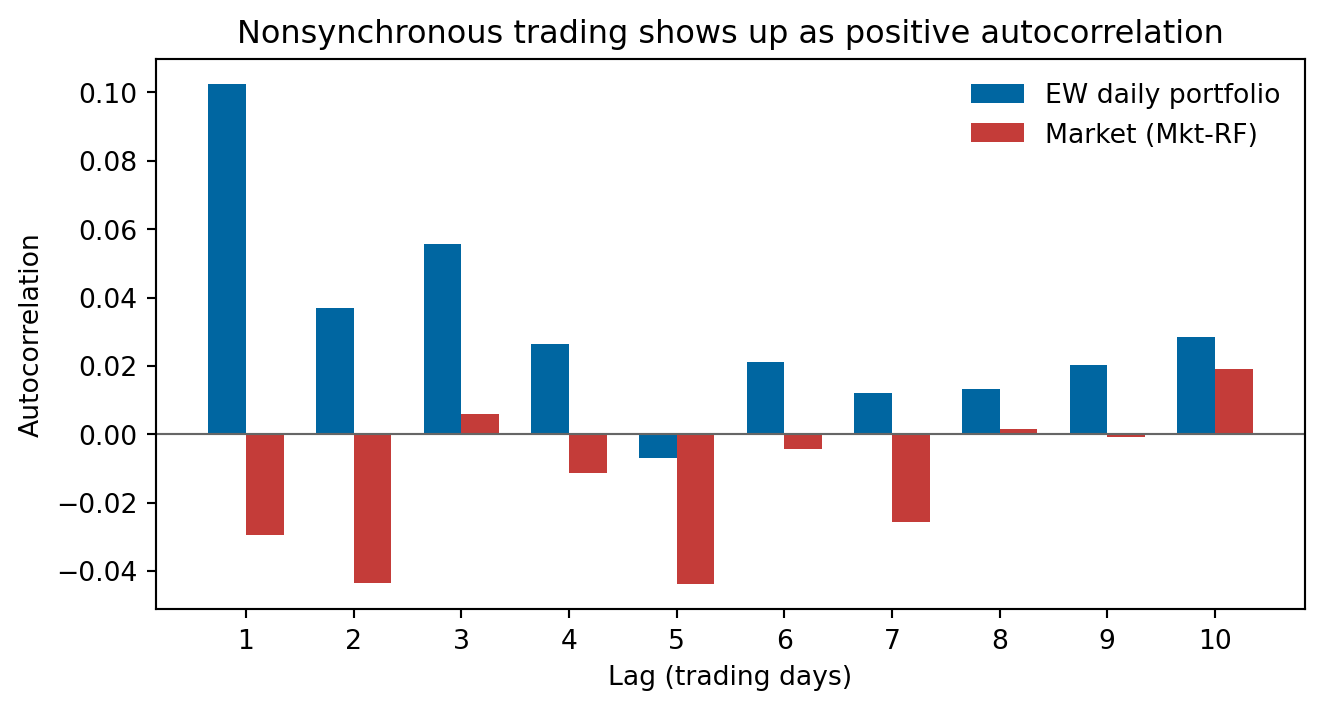
The distribution and zero-density rows are themselves a small confirmation that the pipeline did
something sensible: the market factor, priced almost entirely off the most liquid names on the
exchange, has a handful of exactly-zero days (thin holiday-adjacent sessions); the equal-weighted
portfolio, an average across thousands of names on every day, essentially never lands on an exact
zero. The interesting row is the last one.
```{python}
#| eval: true
#| echo: true
#| fig-height: 3.8
import matplotlib.pyplot as plt

BLUE, RED = "#0066a1", "#c43c39"

def acf(x: np.ndarray, lag: int) -> float:
    return float(np.corrcoef(x[lag:], x[:-lag])[0, 1])

lags = list(range(1, 11))
ew_acf = [acf(ew_ret, l) for l in lags]
mkt_acf = [acf(mkt_rf, l) for l in lags]

fig, ax = plt.subplots(figsize=(7, 3.8))
w = 0.35
ax.bar([l - w / 2 for l in lags], ew_acf, w, label="EW daily portfolio", color=BLUE)
ax.bar([l + w / 2 for l in lags], mkt_acf, w, label="Market (Mkt-RF)", color=RED)
ax.axhline(0, color="#666666", linewidth=0.8)
ax.set_xlabel("Lag (trading days)")
ax.set_ylabel("Autocorrelation")
ax.set_title("Nonsynchronous trading shows up as positive autocorrelation")
ax.set_xticks(lags)
ax.legend(frameon=False)
plt.tight_layout()
plt.show()
```
The equal-weighted portfolio's first-lag autocorrelation sits around $+0.10$; the market factor's
sits slightly *negative*, around $-0.03$. Neither number is a defect in the cleaning pipeline —
both are a real, well-understood feature of averaging many stocks. Not every name in a broad
equal-weighted portfolio trades at the closing instant; yesterday's information keeps arriving in
today's close for the more thinly-traded names, so the portfolio's return has a mechanical echo of
yesterday baked into it, unrelated to any genuine predictability. The market factor, priced off the
most liquid securities on the exchange, does not have this problem, and shows instead the small
negative autocorrelation typically attributed to bid-ask bounce. This is also, concretely, why a
Newey-West standard error matters more for a broad equal-weighted portfolio than for a single
liquid factor — the mechanism this pair of series was originally built to illustrate for Lecture
7's Newey-West material, reused here as a live check on this pipeline's own output.
# What this buys you, and what it doesn't
The eight-filter chain and the decimal correction are good at a specific class of error: one a
statistical pattern can catch without a human ever looking at the specific security. A price or
share count that jumped by an implausible, unconfirmed factor; a security whose typical trading
activity sits in the global bottom 2%; a $(gvkey, iid)$ pair whose economic size just moved in a
way no return or market-equity change backs up. All of these are, in effect, automated tests of
whether an identifier still means "one continuous security" — decimal slips, phantom identity
breaks, and dead-or-illiquid names, at a scale (tens of millions of rows) no human could review by
eye.
What it is not built to catch is anything that requires knowing the specific institutional history
of one security in one country in one month. CLS (2021) are explicit that their own automated
filters leave exactly this residue, which is why Step 8 of their construction exists at all:
> "We investigate and identify in Table 2 errors for Compustat data not captured by the filters
> above."
Table 2 is roughly twenty hand-curated corrections — an Argentine currency-code transition that
manufactures 10,000%-plus returns for four stocks in one month, a Peruvian million-to-one
redenomination Compustat's own feed never caught, an adjustment-factor bug on a single stock's
split. None of these are the kind of thing a threshold or a neighbor-ratio comparison can be built
to find; each one required a human who knew the underlying corporate or monetary event to notice
the number was wrong. That table — not this pipeline — is the right place to look for that class
of error, and `compustat_returns.qmd`'s exercise is where this course teaches it.
The delisting correction is the other capability this pipeline deliberately does not have. The
full `jkp-data` package this construction is ported from *does* include one, in a different module
this port does not use (`gen_delist_df`): `comp.security.secstat == 'I'` (inactive) with
`dlrsni ∈ {'02', '03'}` imputes a $-30\%$ return at delisting, else $0\%$. That rule is BCWX/JKP's
own analogue of the Shumway $-30\%$ imputation the exercise teaches — same headline number, but
keyed on different fields (the *international* `dlrsni` and `secstat`, not the US `dlrsn`/`dldte`
pair on `comp.company` that returns-data-companion.qmd's own delisting section uses) and living in a different
part of the codebase entirely. `bcwx_returns.py`, as documented in this companion, does not inject
it: this pipeline's job is cleaning the rows that exist, not filling in the ones that stopped
existing.
That split — automated pattern-detection on the one hand, a human-curated correction table and a
one-number imputation rule on the other — is really two different philosophies for "fixing the
data," and both are explicit about it. Shumway (1997), building the delisting correction the
exercise teaches, states his own number and its provenance directly:
> "With 71 percent of the delisting returns accounted for, the average return is -30 percent."
and, for researchers who cannot rebuild the underlying over-the-counter dataset:
> "returns of -0.3 replacing the missing performance delisting returns in CRSP."
Shumway & Warther (1999) do the same for Nasdaq, where delisting is both more frequent and more
costly, and are explicit that their number is a constructed hypothetical rather than an average of
observed prices:
> "a corrected return of -55 percent for missing performance-related delisting returns corrects
> the bias" — "4.7 times larger than the delisting bias in NYSE and AMEX data documented by
> Shumway (1997)."
BCWX's decimal correction and eight-filter chain never state a single imputed number anywhere;
every decision is a threshold applied uniformly across tens of thousands of securities, validated
by re-running it against a reference implementation rather than by an economic argument for why
$-30\%$ or $-55\%$ is the right constant. Neither philosophy is strictly better — one scales to a
row count no committee could hand-review, the other captures institutional knowledge no
threshold-based rule could ever encode — and a real returns construction, as CLS's own Table 2
shows, ends up needing both.
::: {.callout-note}
These two Shumway quotes are sourced from `INVENTORY.md`'s pypdf-verified hydration record of
each paper, not from a full split-read `*_text.md` extraction — a minor, stated exception to this
course's usual sourcing discipline, recorded here rather than silently glossed over.
:::
# Sources
- Bessembinder, H., Chen, T.-F., Choi, G. & Wei, K.C.J. (2023). "Long-Term Shareholder Returns:
Evidence from 64,000 Global Stocks." *Financial Analysts Journal*, 79(3). — this repo's code
and output filenames misattribute the paper as "Bessembinder-Cheng-Wei-Xie"; flagged in full
in the private working notes and left uncorrected here.
- Jensen, T. I., Kelly, B. T., & Pedersen, L. H. (2023). "Is There a Replication Crisis in
Finance?" *Journal of Finance*, 78(5), 2465-2518. Code: `bkelly-lab/jkp-data` (MIT license).
Data: `jkpfactors.com` (CC BY-NC).
- Frazzini, A., & Pedersen, L. H. (2014). "Betting Against Beta." *Journal of Financial Economics*,
111(1), 1-25. Cited for the beta estimator this document's re-derive uses, not reproduced here —
see `bab-companion.qmd`'s "The application: the case of the backwards portfolio" for the full
treatment.
- Shumway, T. (1997). "The Delisting Bias in CRSP Data." *Journal of Finance*, 52(1), 327-340.
- Shumway, T., & Warther, V. A. (1999). "The Delisting Bias in CRSP's Nasdaq Data and Its
Implications for the Size Effect." *Journal of Finance*, 54(6), 2361-2379.
- Chaieb, I., Langlois, H., & Scaillet, O. (2021). "Factors and Risk Premia in Individual
International Stock Returns." *Journal of Financial Economics*, 141(2), 669-692, and its Internet
Appendix.
- `returns-data-companion.qmd` (this directory) — the front-half return-construction recap this
document builds on.
- `bab-companion.qmd` (this directory) — the "Building it properly" section this document's
re-derive updates.
- `compustat_returns.qmd` — the tutorial-8
exercise this document is deliberately non-overlapping with (see "What the exercise already
teaches").
```{python}
#| eval: true
#| echo: true
import sys
import numpy as np
import polars as pl
import matplotlib

print("python", sys.version.split()[0])
print("polars", pl.__version__)
print("numpy", np.__version__)
print("matplotlib", matplotlib.__version__)
```