---
title: "Building Gormley–Matsa (2016): Playing It Safe?"
subtitle: "The Lecture 8 Part 1 corporate-finance DiD, assembled from scratch and checked number by number"
format:
html:
toc: true
toc-depth: 2
code-tools: true
code-overflow: wrap
df-print: kable
execute:
warning: false
message: false
eval: false # global default OFF: most chunks read licensed data.
# the five free-data chunks flip eval:true locally.
freeze: true
jupyter: python3 # pipeline is pyfixest/pandas; R cross-checks shown eval:false
---
## How to use this document
Lecture 8's Part 1 works through Gormley and Matsa's *Playing It Safe? Managerial
Preferences, Risk, and Agency Conflicts* (*Journal of Financial Economics*, 2016): the
staggered state adoption of business-combination antitakeover laws, and what insulated
managers do with the firm's cash and risk. The slides show results and hide the code; this
document does the opposite, rebuilding the whole replication in the order the lecture tells
it and printing our reproduced number next to the paper's for every claim.
Unlike the Olken replication that sits behind this course's other Lecture 8 companion, this
one cannot run end to end on your laptop. Gormley–Matsa rests on Compustat `funda`/`fundq`
(and, for the risk legs, `secd`-derived daily returns): licensed instructor data that is
gitignored and never redistributable. So the WRDS pulls and every regression that reads the
built panel are shown but not executed (`eval: false`), and their outputs are quoted from
the pipeline's frozen ledgers in `outputs/`. Exactly one input is free and public — the
33 business-combination-law adoption years, hand-coded from Gormley–Matsa's Appendix Table
A.1 — so the treatment indicator, the cohort map, and a small piece of arithmetic *do* run,
and the two robustness figures rebuild live from committed result ledgers.
Five code chunks in this document execute: the BC-dates spine (§1), the log-points
arithmetic (§8), the leave-one-out figure (§13), the standard-error-versus-N figure (§16),
and the session-info footer. Everything else is displayed for reading, with its result
quoted from a named ledger cell. The [pipeline map](#the-pipeline-at-a-glance) below says
which script produces which number, and whether it runs here.
Two panel vintages appear throughout, and they are never silently mixed. The **1976–2006
baseline** is Gormley–Matsa's own window; the cash and bad-controls legs are quoted on it so
they sit against the paper's own N. The **extended 1976–2026 vintage** re-runs the same
scripts with the sample end pushed to today; the volatility legs are quoted on it because
that is where they reach the paper's sample size. Every table below carries both, side by
side, and names its window.
## The pipeline at a glance {#the-pipeline-at-a-glance}
The build is a small directed graph of scripts. Only the first row and the three figure
rows touch no licensed data; everything else reads a gitignored Compustat extract and is
shown, not run, with its numbers quoted from the ledger it writes.
| Script | Reads | Produces | Runs here? |
|---|---|---|---|
| `code/gm_bc_dates.py` | GM Appendix Table A.1 (printed) | `data/gm_bc_dates.csv` — 33 state→year pairs, treatment rule, cohort map | **yes** (free) |
| `pull_compustat_gm.py` | WRDS `comp.funda ⋈ comp.company` | `data/gm_compustat_raw.parquet` (gitignored) | no (`eval:false`) |
| `pull_compustat_gm_fundq.py` | WRDS `comp.fundq` | `data/gm_fundq_raw.parquet` (gitignored) | no (`eval:false`) |
| `code/gm_did.py` | built panel | `outputs/gm-pipeline-numbers.md` (G1–G9, B1–B3) + `gm_event_study_cash.png` | no (`eval:false`) |
| `code/gm_de_robustness.py` | built panel | `outputs/gm-de-robustness.md` (G12, G12b) | no (`eval:false`) |
| `code/gm_cashflow_vol.py` | panel + `fundq` | `outputs/gm-cashflow-vol.md` (G5) | no (`eval:false`) |
| `code/gm_stock_vol.py` (+ probe) | panel + BCWX/JKP daily | `outputs/gm-stock-vol.md` (G10, G11) | no (`eval:false`) |
| `gm_did_rcheck.R`, `gm_phase3_rcheck.R` | built panel | R `fixest` cross-checks | no (`eval:false`) |
| `code/gm_fig_adoption_timing.py` | `gm_bc_dates` + one quoted share | `figures/gm_adoption_timing.png` | figure (free) |
| `code/gm_fig_leaveoneout.py` | `outputs/gm-de-robustness.md` | `figures/gm_leaveoneout.png` | **yes** (parses ledger) |
| `code/gm_fig_se_vs_n.py` | `outputs/gm-cornerstone-findings.md` | `figures/gm_se_vs_n.png` | **yes** (ledger numbers) |
The three "runnable" figures do not recompute any regression: two of them rebuild the
picture from a frozen result ledger, and the adoption-timing figure draws only the printed
dates. Read them as *renders of committed results*, not fresh estimation.
## 1. The one shareable input: BC-law adoption dates
Everything downstream keys off a single, entirely public fact: which state adopted a
business-combination law in which year. Gormley–Matsa print these in Appendix Table A.1, so
they carry no licence. `code/gm_bc_dates.py` transcribes that table into a state→year
lookup and a treatment rule, and it is the one piece of this build a student can run.
```{python}
#| eval: true
#| echo: true
import sys, os
import pandas as pd
sys.path.insert(0, "code")
import gm_bc_dates as bc

# 33 adopting states, keyed to state of INCORPORATION, sorted by adoption year.
dates = (
    pd.DataFrame(
        [(s, bc.STATE_NAMES[s], y,
          "Pinnell 2000" if s in bc.PINNELL_ADDITIONS else "Bertrand–Mullainathan 2003")
         for s, y in bc.BC_LAWS.items()],
        columns=["state", "name", "adopt_year", "source"],
    )
    .sort_values(["adopt_year", "state"])
    .reset_index(drop=True)
)
dates
```
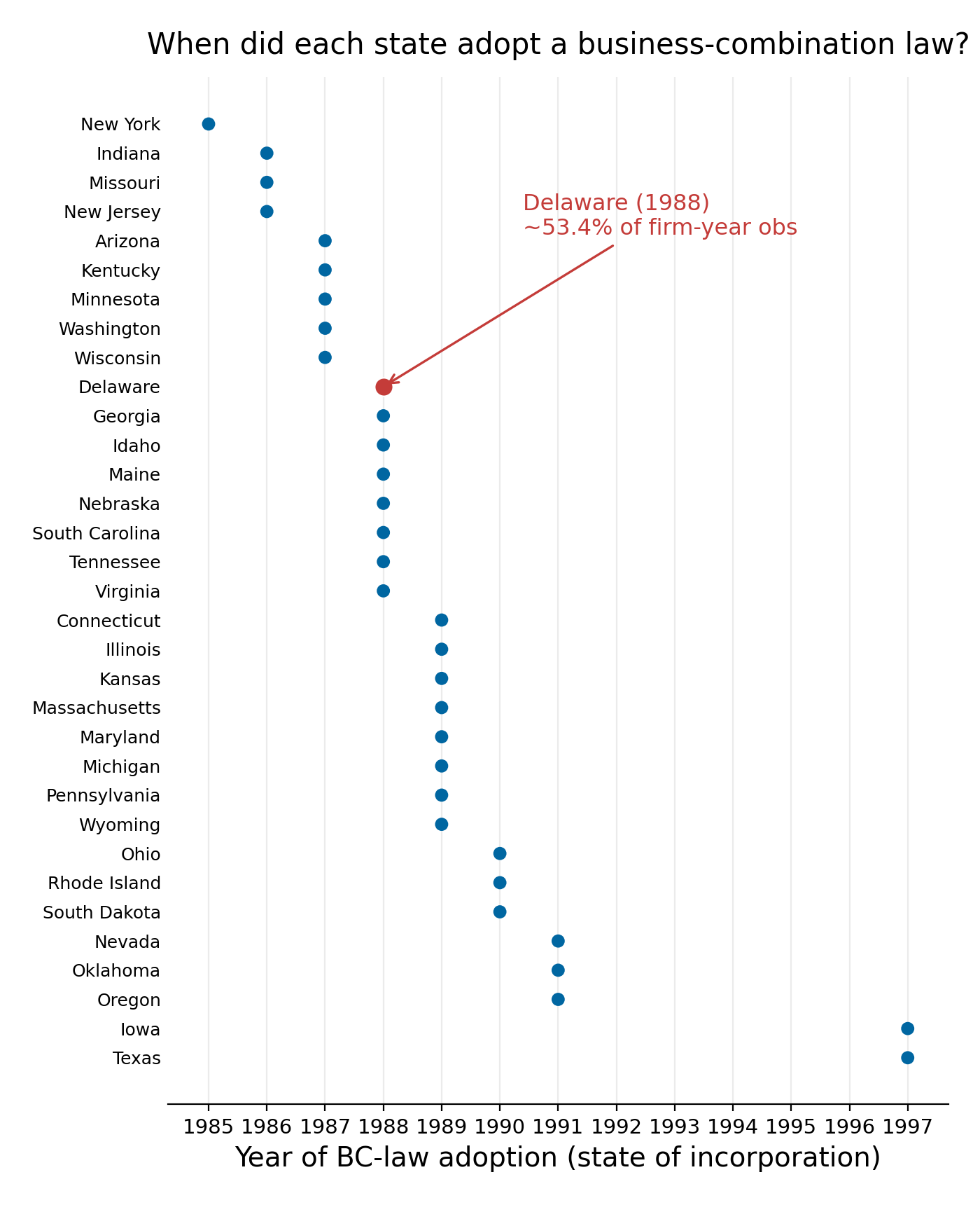
The roster runs from New York in 1985 to Iowa and Texas in 1997 — 33 states in all. Thirty
of them are the Bertrand–Mullainathan (2003) set that adopted between 1985 and 1991;
Gormley–Matsa add three more from Pinnell (2000) — Oregon (1991), Iowa and Texas (both
1997). The absorbing treatment dummy switches on in a firm's adoption year and stays on, and
firms incorporated in a never-adopting state (Florida, California) are never treated:
```{python}
#| eval: true
#| echo: true
checks = {
    "DE treated in 1987 (before its 1988 law)": bc.is_treated("DE", 1987),
    "DE treated in 1988 (adoption year)":       bc.is_treated("DE", 1988),
    "FL treated in 2000 (never adopts)":        bc.is_treated("FL", 2000),
    "states in the full set":                   len(bc.BC_LAWS),
    "states in the BM-only 30-state subset":    len(bc.bm_only()),
}
checks
```
The `bm_only()` subset drops the three Pinnell additions to recover the core 30-state
Bertrand–Mullainathan design the literature standardised on — a robustness leg we return to
in §7. The treatment is assigned on the firm's **state of incorporation**, which is the
whole design and the subject of the next section. In the paper's own words on what the laws
reach:
> These state laws applied only to target firms incorporated in the state.
and, from footnote 1,
> the BC laws make only hostile takeovers of target firms incorporated in that state more
> difficult. Friendly mergers are unaffected by the law, as are hostile takeovers of firms
> incorporated elsewhere, even when the acquirer is incorporated in the affected state.
The timing is easiest to read as a strip. Delaware — the dot to watch, because it carries
**53.4% of firm-year observations** in the baseline panel (`gm-pipeline-numbers.md` §G1) —
adopts in 1988. The figure below is drawn by `gm_fig_adoption_timing.py`, which needs only
the dates above plus that one quoted share; it is committed and regenerable, shown here as a
static image.
{fig-align="center" width="70%"}
## 2. Incorporation versus location: where identification comes from
Treatment follows the state a firm is *incorporated* in, not the state where it operates —
and those come apart. More than 60% of firms incorporate and locate in different states, and
that gap is the entire identification argument. Because incorporation and location are
distinct, the regression can absorb everything that hits a *location* in a given year
(local business cycles) and everything that hits an *industry* in a given year, and still
have treatment variation left to read. In the authors' words:
> Using a difference-in-differences estimator, we compare changes among firms located in
> states that pass a BC law with changes among firms incorporated elsewhere. The underlying
> identification assumption is that, but for the law, the two sets of firms would follow
> parallel trends; that is, the change in outcome $y$ for firms incorporated in the states
> that pass a BC law would have been the same as for firms incorporated in states that did
> not pass a BC law.
and the sentence that licenses the state-by-year fixed effects:
> We are able to obtain estimates for the BC laws' effects even after including
> state-by-year fixed effects because more than 60% of our firms are incorporated and
> located in different states. Our estimates are identified by comparing the differential
> response of two firms that operate in the same state, $l$, but when only one of these
> firms is incorporated in a state, $s$, that passes a BC law. Thus, any unobserved,
> time-varying state-level factors, such as local business cycles, that could coincide with
> a BC law's adoption and affect our outcomes of interest do not bias our findings.
::: {.callout-note title="The 2×2, and why location does not confound it"}
Two firms in the same building in Palo Alto, selling to the same customers, in the same
industry:
| Firm | Incorporated in | Operates in | Treated from |
|---|---|---|---|
| A | Delaware | California | 1988, when Delaware adopts |
| B | California | California | never — California does not adopt |
A California-by-year shock hits both identically and is swept out by the location-by-year
fixed effect. What remains is that one of them was treated in 1988 because of a filing
cabinet in Wilmington. That is the variation the design uses.
:::
The >60% figure is Gormley–Matsa's own (`gm-cornerstone-expectations.md`, "What we
reproduce"); we do not recompute it here, because doing so needs the Compustat header that
carries incorporation and location state.
## 3. Recall the week-6 machinery
Nothing in the estimand is new this week. The target is the average treatment effect on the
treated,
$$
\text{ATT} = E\!\left[\,Y_{it}(1) - Y_{it}(0)\;\middle|\;W_{it}=1\,\right],
$$
with $Y_{it}(1)$ and $Y_{it}(0)$ the two potential outcomes for firm $i$ in year $t$ and
$W_{it}$ the treatment indicator. It is identified under the four week-6 assumptions —
consistency, no anticipation, no interference, and parallel trends — the last of which
Gormley–Matsa state exactly as the "but for the law … the two sets of firms would follow
parallel trends" sentence quoted above. The one genuinely new object is that $W_{it}$
switches on at a *different date for different firms*: **staggered** adoption. A single
before-after 2×2 becomes a stack of them, one per adoption cohort, and that stack is where
the staggered-DiD problems of §12 come from. Everything from §4 onward is week-6 machinery
run on real data.
## 4. Assembling the panel from Compustat
The panel is a WRDS pull followed by a handful of sample screens. The pull joins
`comp.funda` to the `comp.company` header for the incorporation and location states, and —
crucially — applies **no common-stock or size screen**. That absence is deliberate: it is
the whole reason this cornerstone reproduces where a CRSP-screened one attenuates
(§18 returns to that contrast). The complete, runnable pull is `pull_compustat_gm.py`; its
core query, shown but not executed here:
```{python}
#| eval: false
#| echo: true
# pull_compustat_gm.py — WRDS Compustat annual pull (INSTRUCTOR-DATA, gitignored).
# No CRSP, no common-stock screen. Treatment/cluster key is c.incorp; the
# location-by-year FE uses c.state (HQ). Runnable with WRDS access:
#   (the pull script lives in the private working repo; not shipped here)
import wrds
conn = wrds.Connection(wrds_username=os.environ["WRDS_USER"])
df = conn.raw_sql("""
    select f.gvkey, f.fyear, f.datadate, f.sich,
           f.at, f.sale, f.ni, f.ch, f.che,
           f.dltt, f.dlc, f.lt, f.re, f.wcap, f.oiadp,
           f.csho, f.prcc_f, f.dvc, f.prstkc, f.act, f.lct, f.dp,
           c.incorp as inc_state,   -- TREATMENT: state of incorporation
           c.state  as hq_state,    -- location, for the location-by-year FE
           c.loc    as hq_loc, c.sic as header_sic
    from comp.funda f
    left join comp.company c on f.gvkey = c.gvkey
    where f.indfmt='INDL' and f.datafmt='STD' and f.popsrc='D' and f.consol='C'
      and f.fyear between 1974 and 2026 and f.at is not null and f.at > 0
""")
```
The screens Gormley–Matsa describe are applied downstream in `gm_did.py`, so the drop counts
stay visible. In the paper's own statement of them:
> We obtain firms' financial data from Compustat, excluding regulated utility firms (SIC
> codes 4900–4999), firms located or incorporated outside the US, and firm-year observations
> with either missing or negative assets or sales. Financial ratios are winsorized at the 1%
> level. To include at least ten years of data before and after each law's adoption, our
> sample period is 1976–2006.
and, on the endogeneity of incorporation itself:
> To avoid endogenous changes in whether a firm is subject to a BC law, we exclude firms
> that reincorporate from a state without a BC law to a state with a BC law or vice versa.
Our build uses the *current* Compustat incorporation header rather than Gormley–Matsa's
historical (Cohen 2012) coding. Their footnote 6 settles that this is immaterial:
> Relative to the most recent version of Compustat, our historical data change the state of
> incorporation for about 6% of observations and change treatment status for only 2% of
> observations.
so the current-header build is Gormley–Matsa's own stated robustness variant. The build code,
shown but not executed:
```{python}
#| eval: false
#| echo: true
# gm_did.py — build_panel(): screens, outcomes, treatment (INSTRUCTOR-DATA).
df = df[df["hq_loc"] == "USA"]
df = df[df["inc_state"].isin(US_STATES) & df["hq_state"].isin(US_STATES)]
df["sic4"] = pd.to_numeric(df["sich"].fillna(df["header_sic"]), errors="coerce")
df = df[~df["sic4"].between(4900, 4999)]           # utilities only (GM keeps financials)
df = df[(df["at"] > 0) & (df["sale"] > 0)]
df["ln_cash"] = np.log(df["ch"].where(df["ch"] > 0))   # ln(ch); ch>0 only
df["cash_at"] = df["che"] / df["at"]
for c in ["cash_at", "ch_at", "roa", "debt_at", "payout_at"]:
    df[c] = winsorize(df[c], 0.01, 0.99)               # ratios winsorized 1/99
df["bc"] = [is_treated(s, int(y)) for s, y in zip(df["inc_state"], df["fyear"])]
df["bc_cohort"] = df["inc_state"].map(adoption_year)   # cohort = adoption year
```
The resulting sample is quoted below on both vintages (`gm-pipeline-numbers.md` §G1 and
`gm-pipeline-numbers-2026.md` §G1). A student who checks GM's location assignment will find
it is the headquarters — "We assign a firm's location based on the location of its
headquarters, which is typically also where major plants and operations are located."
| | 1976–2006 baseline | Extended to 2026 |
|---|---|---|
| Ln(cash) firm-years | **174,627** (GM 172,739; within 1.1%) | 262,641 |
| Unique firms | 17,837 | 22,266 |
| Treated incorporation-states | 33 | 33 |
| Never-treated firm-years | 18,639 | 24,522 |
| Delaware share of observations | 53.4% | 55.8% |
The extension adds only post-treatment and never-treated mass — every adoption is 1985–1997 —
so it introduces no new staggered-timing comparisons, only more data of the kinds already
present.
## 5. From the 2×2 to the regression we run
The design maps onto two specifications, worth seeing side by side because the contrast
between them *is* the identification lesson. The teaching baseline is the week-4/week-5 two-way
fixed-effects model,
$$
Y_{it} = \alpha_i + \lambda_t + \delta\,W_{it} + u_{it},
$$
firm and year fixed effects with one treatment dummy. Gormley–Matsa's own specification
replaces the year effect with location-state-by-year and four-digit-industry-by-year effects
(their Eq. 4):
$$
y_{ijlst} = \beta_1\,BC_{st} + f_i + \omega_{lt} + \lambda_{jt} + \eta_{ijlst},
$$
which the authors read out as:
> $f_i$ are firm fixed effects; $\omega_{lt}$ are state-by-year fixed effects; and
> $\lambda_{jt}$ are four-digit SIC industry-by-year fixed effects. … Finally, we adjust the
> standard errors for clustering at the state-of-incorporation level.
The extra structure is exactly what the incorporation-versus-location gap pays for, and it is
what makes the heavy-FE estimate defensible:
> The inclusion of state-by-year and industry-by-year fixed effects ensures that our
> difference-in-differences estimates are robust to many types of unobservable omitted
> variables that could otherwise confound our analysis.
Two choices carry the weeks-1-through-5 material into this design. First, the standard errors
cluster on **state of incorporation** — the level treatment is assigned at, the clustering
lesson from `lecture4.qmd` used in anger, and the number that comes back to bite us in §16.
Second, there are **no firm controls** in the headline: no size, no leverage, no
profitability on the right-hand side. That is deliberate, and §14 is its defence. In
`pyfixest`, the headline is one line:
```{python}
#| eval: false
#| echo: true
# gm_did.py:143 — paper FE spec, clustered on incorporation state (INSTRUCTOR-DATA).
import pyfixest as pf
FE_PAPER = "gvkey + hq_state^fyear + sic4^fyear"     # firm + loc-state×year + sic4×year
m = pf.feols("ln_cash ~ bc | " + FE_PAPER, data=d_cash, vcov={"CRV1": "inc_state"})
```
## 6. Threats, named before results
Four ways this could be wrong, named before a single estimate appears — a commitment device
that stops the diagnostics from being chosen after the fact to flatter the result. Three of
the four are omitted-variable stories in the weeks-1-2 sense: something left out that
correlates with both treatment and cash. The fourth is the mirror image, and the one students
most often get wrong: a variable wrongly *put in*, one the treatment itself moves.
| # | Threat | The story | Answered in |
|---|---|---|---|
| i | Pre-existing drift | cash was already trending up in treated states before adoption | §10 (event study), §11 (placebo) |
| ii | Staggered contamination | already-treated firms used as controls for later cohorts (Goodman-Bacon) | §12 (Sun–Abraham) |
| iii | A dominant cohort | Delaware alone is 53% of the file and adopts in 1988 | §13 (drop DE, leave one out) |
| iv | Bad controls | conditioning on size/leverage/ROA, which the law itself moves | §14 |
Gormley–Matsa's own defence against threat (i)/(iii)-style legislative endogeneity leans on
the political economy of the laws:
> Romano (1987) and Bertrand and Mullainathan (2003) find that the passage of these laws
> typically did not result from the pressure of a large coalition of economic players in the
> state and conclude that an omitted economic variable is unlikely to explain measured
> effects of the law.
and on a five-part run of evidence they summarise as:
> First, we find no measureable differences in the ex ante characteristics of firms
> incorporated in states adopting the laws. Second, no preexisting trends exist … before the
> laws come into effect. … All five of these results suggest that our findings are not
> explained by legislative endogeneity.
Each threat gets its own section, in the order above, and each answer is reported whether or
not it is comfortable.
## 7. The headline: what the paper found, and what the rebuild found
Same law, same window, an independently assembled Compustat extract. The sample lands within
1.1% of the paper's, the coefficient at 89% of theirs, and — the detail worth dwelling on —
estimated *more precisely than the paper's own* (t 2.89 against 2.47). Numbers from
`gm-pipeline-numbers.md` §G1/§G2/§G3/§G8 and `gm-cornerstone-findings.md`, headline verdict;
extended column from `gm-pipeline-numbers-2026.md`.
| | GM (2016), Table 2 | Rebuild, 1976–2006 | Rebuild, extended 2026 |
|---|---|---|---|
| Ln(cash), N | 172,739 | **174,627** (within 1.1%) | 262,641 |
| **Ln(cash)** | **+0.121 (t 2.47)** | **+0.1081** (SE 0.0374, t **2.89**, p .006) | +0.1057 (SE 0.0408, t 2.59, p .013) |
| Cash ratio, che/at | +0.0023, ns | −0.0024 (SE 0.0027, t −0.90) | −0.0018 (t −0.68) |
| BM-only 30-state | ≈ +0.121 | **+0.1225** (t 2.77) | +0.1194 (t 2.44) |
| Alternative timing (first full year) | — | +0.0624 (t 1.68) | +0.0614 (t 1.52) |
The closest apples-to-apples row is the last-but-one: dropping the three Pinnell late-adopters
(Iowa, Oregon, Texas) to recover Gormley–Matsa's core 30-state Bertrand–Mullainathan design
gives **+0.1225 (t 2.77)**, a whisker from the paper's +0.121. A replication that lands within
one percent on sample size has the same firms in it, which is what licenses reading the
coefficient comparison at all.
The estimate is identical in R. `gm_did_rcheck.R` re-runs the same built panel through
`fixest::feols` and reproduces `pyfixest` to the reported precision:
::: {.panel-tabset}
## Python (`pyfixest`)
```{python}
#| eval: false
#| echo: true
m = pf.feols("ln_cash ~ bc | gvkey + hq_state^fyear + sic4^fyear",
             data=d_cash, vcov={"CRV1": "inc_state"})
# -> bc = +0.1081, t 2.89, N 174,627   (gm-pipeline-numbers.md §G2)
```
## R (`fixest`)
```r
# gm_did_rcheck.R — reads the identical built panel Python used.
library(fixest); library(arrow)
d <- as.data.frame(read_parquet("data/gm_panel_built.parquet"))
d <- d[!is.na(d$ln_cash), ]
m_paper <- feols(ln_cash ~ bc | gvkey + hq_state^fyear + sic4^fyear,
                 data = d, cluster = ~inc_state)
# -> beta +0.1081, t 2.89, N 174,627   (matches pyfixest exactly)
```
:::
One sentence on *why this paper*: Gormley–Matsa's cash sample is Compustat-native with no
common-stock screen, so it structurally escapes the CRSP-screen attenuation that hit the
runner-up cornerstone (Serfling 2016) on the same install (`gm-cornerstone-findings.md`,
Serfling comparison) — the reason it was chosen over an otherwise-similar staggered-law
design.
## 8. Reading the coefficient
The headline is on log cash, so exponentiating turns it into a percentage. This is pure
arithmetic on printed coefficients — no data — so it runs:
```{python}
#| eval: true
#| echo: true
import numpy as np
import pandas as pd

pd.DataFrame({
    "source":        ["Rebuild (1976–2006)", "GM (2016) printed"],
    "beta_ln_cash":  [0.1081, 0.121],
    "pct_change":    [np.exp(0.1081) - 1, np.exp(0.121) - 1],
}).assign(pct_change=lambda d: (d["pct_change"] * 100).round(1))
```
So $\exp(0.1081)-1 \approx 11.4\%$ more cash, against Gormley–Matsa's own 12.1 log points,
"or about 13%." Insulated managers hold more cash — precautionary hoarding, or a quiet life;
this lecture does not adjudicate between those stories and should not pretend to. The caveat
arrives immediately, in the next section: the cash *ratio* does not move.
## 9. Log-level versus ratio: the same data, two answers
Cash grew. So did assets. Which normalisation gets used is a modelling choice with a real
answer attached, not a formatting detail — and here the two choices disagree.
Numbers from `gm-pipeline-numbers.md` §G3 (extended column §G3 of the 2026 file).
| Outcome | Rebuild, 1976–2006 | Rebuild, extended 2026 | GM (2016), printed |
|---|---|---|---|
| **Ln(cash)** | **+0.1081** (t 2.89), N 174,627 | +0.1057 (t 2.59) | +0.121 (t 2.47) |
| Cash ratio che/at | −0.0024 (SE 0.0027, t −0.90), N 193,261 | −0.0018 (t −0.68), N 283,331 | +0.0023 (SE 0.0034), ns |
| Cash ratio ch/at | +0.0013 (t 0.51) | +0.0015 (t 0.54) | — |
The disagreement is not a replication failure: Gormley–Matsa's own printed ratio result is
null too. In their words,
> Average total cash holdings increase by 12.1 log points, or about 13%, after a BC law is
> adopted (Column 5), but the increase in the ratio of cash to book assets is smaller and not
> significant (coefficient = 0.0023, standard error = 0.0034).
So both builds say the same thing — the *level* of cash moves and the *share* of the balance
sheet held as cash does not — which means assets grew roughly in step with cash. Whether that
is the interesting fact or a nuisance depends entirely on the question. A student who reports
only the specification that moved has not made a coding error; they have made a write-up
error.
::: {.callout-note title="Why the sample sizes differ"}
The three cash rows run on different N: Ln(cash) needs `ch > 0` (193,261 firm-years have a
defined cash ratio, but only 174,627 have positive cash to log), and the ratio uses the full
defined sample. This is the same reason the §11 placebo (56,006) and the headline (174,627)
differ — different rows are eligible for different questions. Naming the estimation sample is
part of naming the estimate.
:::
## 10. Pre-trends: the event study GM never drew
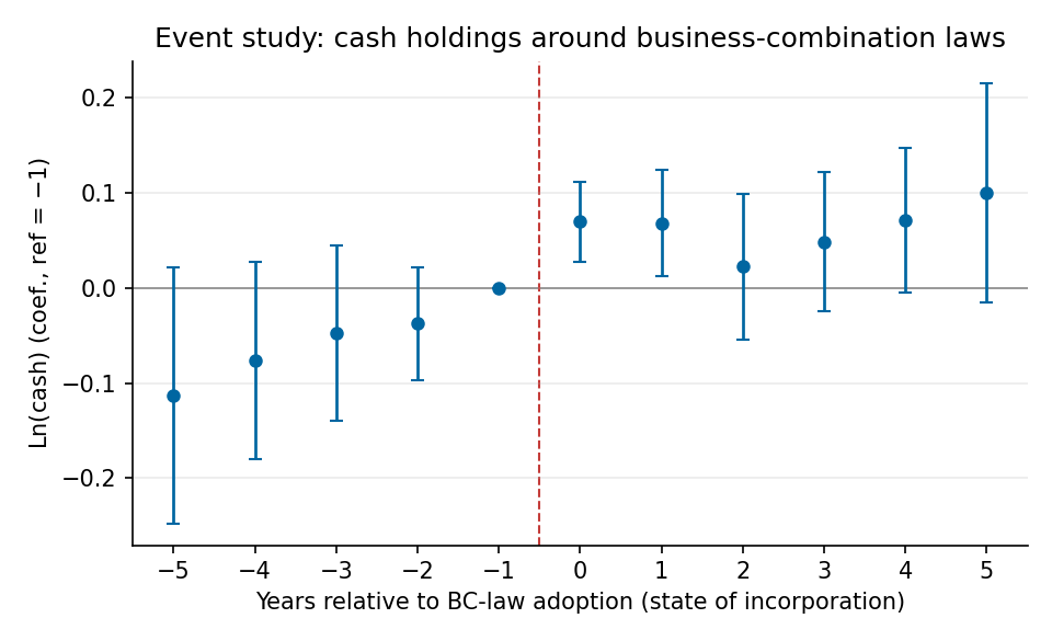
Gormley–Matsa plot acquisitions, not cash — their Figure 2 is the acquisition event study,
and nobody draws the cash pre-trend. So we did. The figure below (from `gm_did.py`, static;
its source needs the licensed panel and is not regenerated here) puts the reference year at
$k=-1$ and reads the leads. Numbers from `gm-pipeline-numbers.md` §G6/§G7.
{fig-align="center" width="72%"}
The leads all clear the bar — $t$ of $\{-5:-1.64,\ -4:-1.45,\ -3:-1.00,\ -2:-1.26\}$, every
$|t|<1.65$ — which is the parallel-trends evidence the paper never shows for cash. But the
honest beat is that every lead sits *mildly negative*, and $k=-5$ is a whisker from the line
at $-1.64$: a faint hint of an upward cash drift into adoption. Not a violation; the "is this
pre-trend real?" moment. After adoption the effect is immediate and sustained — $k=0$ at
**+0.0696 (t 3.2)**, holding to $k=5$ at **+0.1002** — but it dips at $k=2$ (+0.0225) rather
than phasing in monotonically.
::: {.callout-warning title="Logged honestly as CHECK, not PASS"}
The dynamics are an immediate, persistent, growing increase, but *not* a strict monotone
phase-in. The pipeline records G7 as **CHECK**, and this document does not launder it to PASS.
Gormley–Matsa's own timing claim is the qualitative one this supports: "the law's adoption
precedes the effects we assign to it instead of the other way around."
:::
## 11. The placebo, reported honestly
Move every adoption three years earlier and estimate on the pre-period alone. Nothing happened
in those years, so the coefficient should be zero. It is insignificant — **+0.0591 (t 1.68),
N 56,006** (`gm-pipeline-numbers.md` §G9; extended: +0.0603, t 1.65, N 61,889) — but it leans
positive, in exactly the direction the mild leads of §10 hinted at.
A placebo that "passes" at 1.96 and a pre-trend that "passes" at 1.65 can be telling you the
same soft thing. "The placebo is insignificant" is a true sentence and an incomplete one; the
reader is owed the coefficient, the $t$, and the direction it leans. This is the same
report-don't-launder discipline the pre-testing literature (week 6) asks for.
## 12. Staggered timing is not one experiment
With 33 treated cohorts and a thin never-treated group, the static two-way fixed-effects
coefficient is exposed to the Goodman-Bacon problem: some of its identifying 2×2s use
already-treated firms as controls for later-adopting ones, a comparison nobody intended. The
structure is visible from the shares alone (`gm-pipeline-numbers.md` §B1): **33 treated
incorporation-states versus 18 never-treated**; treated-state firm-years **89%** against
**11%** never-treated; and Delaware alone is **53% of observations, adopting in 1988**, so the
DE-1988 cohort's 2×2s carry heavy weight while the clean control group is small. Exact
Goodman-Bacon weights need a balanced panel, so this is kept qualitative; the quantitative
answer is the heterogeneity-robust estimator, whose natural tool here is Sun–Abraham
(`fixest::sunab`).
::: {.panel-tabset}
## R (`fixest::sunab`)
```r
# gm_did_rcheck.R — Sun-Abraham event study, never-treated as control.
d$cohort <- ifelse(is.na(d$bc_cohort), 10000, d$bc_cohort)
m_sa <- feols(ln_cash ~ sunab(cohort, fyear) | gvkey + fyear,
              data = d, cluster = ~inc_state)
aggregate(m_sa, agg = "att")
# -> ATT +0.169 (SE 0.0507, t 3.33, p .0016); path k0..k5 +0.093 → +0.088
```
## Python (hand-rolled)
```{python}
#| eval: false
#| echo: true
# gm_did.py — cohort × relative-time saturated design, never-treated control.
# Overall post ATT (cohort-share weighted) = +0.1012
# path k0..k5: +0.0999, +0.0820, +0.0674, +0.0883, +0.1326, +0.1369
```
:::
Both implementations survive: the aggregate ATT is positive and significant, and the
event-time path is positive and roughly flat under each (`gm-pipeline-numbers.md` §B2, R
cross-check). The two aggregates differ — Python's **+0.1012** against R's **+0.169
(t 3.33, p .0016)** — because of aggregation weighting and endpoint binning, not because one
is wrong.
::: {.callout-important title="Report the sign and the path, never one SA number"}
A heterogeneity-robust estimate is a *family* of estimates; quoting one of them to three
decimal places as "the answer" overstates what the method delivers. The teachable fact is
that the sign and the path survive the correction — the static coefficient was not an artefact
of forbidden comparisons.
:::
This is the one diagnostic with no Gormley–Matsa quote: the paper predates the
staggered-DiD critique, so the estimator is attributed to Sun & Abraham (2021) and this
companion, not to the original.
## 13. Kill the dominant cohort: drop Delaware, then leave one state out
Delaware is 53% of the sample and adopts in 1988, so the single most direct robustness check
is to remove it entirely and see if the result dies. It does not (`gm-de-robustness.md` §G12):
dropping Delaware takes N from 174,627 to **81,345** and gives paper-FE Ln(cash) **+0.1429
(SE 0.0667, t 2.14, p .037)** — positive, still significant, and in fact *larger* than the
full-panel +0.1081, because the heavy fixed-effect structure no longer competes with the
dominant cohort for the same variation (the firm+year baseline on the DE-excluded sample is
+0.1470, t 2.94). This matches Gormley–Matsa's own §6.4, and their summary of the whole
robustness family:
> Finally, our findings are robust to alternative samples, time periods, and empirical
> specifications, including excluding firms incorporated in Delaware (50% of observations) or
> any of the 32 other states that adopted a BC law.
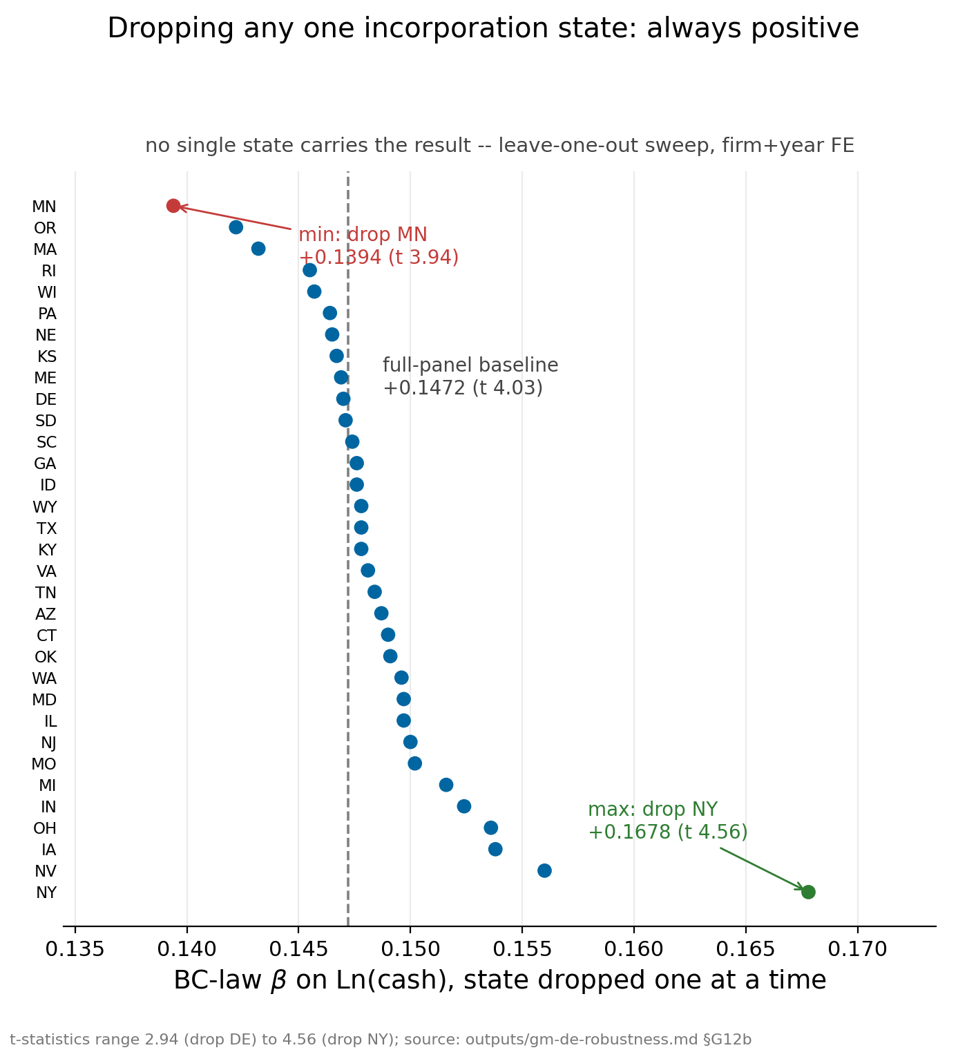
That last clause — *any of the 32 other states* — is the leave-one-out sweep, which the
pipeline runs and which this document rebuilds live. `gm_fig_leaveoneout.py` parses the
33-row table straight out of the committed ledger (it asserts exactly 33 rows, so a drifted
ledger fails loudly) and plots the firm+year-FE coefficient with each treated state dropped in
turn:
```{python}
#| eval: true
#| echo: true
import contextlib, io
sys.path.insert(0, "code")
import gm_fig_leaveoneout
with contextlib.redirect_stdout(io.StringIO()):
    gm_fig_leaveoneout.main()   # rebuilds the figure from outputs/gm-de-robustness.md
from IPython.display import Image
Image("outputs/figures/gm_leaveoneout.png")
```
Across all 33 states the coefficient stays in **[+0.1394, +0.1678]** and never changes sign —
minimum when Minnesota is dropped (+0.1394, t 3.94), maximum when New York is dropped (+0.1678,
t 4.56), against a full-panel firm+year baseline of +0.1472 (`gm-de-robustness.md` §G12b). The
punchline is a sentence students can reuse in any staggered design: identification does not
rest on any single treated unit, and if it does, that is a finding about the paper, not about
the world.
## 14. Bad controls versus AvgE: two ways to break a clean estimate
The absence of firm controls in the headline (§5) was deliberate, and this is its defence.
Size, leverage and profitability are all things a business-combination law can move, so
conditioning on them shuts down part of the very channel being measured. Gormley–Matsa's
literal demonstration of this (their Table 7) is on the number of acquisitions — an SDC-gated
outcome we cannot build — so the lesson is run here on Ln(cash) instead, where *both*
directions of bias show up on a single outcome (`gm-pipeline-numbers.md` §B3, extended §B3).
| Specification | 1976–2006 | Extended 2026 |
|---|---|---|
| Proper FE, no controls | **+0.1081** (t 2.89, N 174,627) | +0.1057 (t 2.59) |
| + endogenous "bad controls" (log assets, leverage, ROA) | **+0.0795** (t 3.18, N 174,624) | +0.0698 (t 2.60) |
| AvgE "common error" (group-mean DV in place of FE) | **+0.1942** (t 6.68, N 174,627) | +0.2357 (t 9.56) |
Post-treatment mediators attenuate the estimate by about 26%; the "AvgE" substitution
documented in Gormley & Matsa's (2014) *Common Errors* — replacing the fixed effects with a
group average of the dependent variable, which looks like a control and is not — inflates it
by about 80%. Bias runs in both directions from one clean estimate.
::: {.callout-important title="The detail that lands hardest"}
Read the $t$ column top to bottom: 2.89, then 3.18, then 6.68. Both mistakes make the result
look *better* — tighter, more publishable. A rising t-statistic is not evidence that a
specification improved. The exam-shaped rule: a control that the treatment itself moves is not
a control; it is part of the effect being measured (Angrist–Pischke on bad controls; Gormley &
Matsa 2014).
:::
## 15. Did they actually get safer? Three risk measures
Gormley–Matsa's substantive claim is that insulated managers take less risk. Three measures
test it, and they return three different verdicts. Two of the three are built from
Compustat-`secd`-derived daily returns with **no CRSP anywhere in the pipeline** — the
deliberate stress test, since Gormley–Matsa build their volatility from CRSP. Quoting GM's own
"from CRSP" beside our no-CRSP build is what makes the stress explicit.
Both vintages, from `gm-cashflow-vol{,-2026}.md` and `gm-stock-vol{,-2026}.md`:
| Measure | Rebuild, baseline | Rebuild, extended 2026 | GM (2016) | Verdict |
|---|---|---|---|---|
| Cash-flow volatility | −0.0015 (t −0.92), N 102,153 | −0.0024 (t −1.05), N 159,268 | −0.0028, ns | null reproduced — **PASS** |
| Stock volatility | −0.0172 (t −2.26), N 81,936 | **−0.0232** (SE 0.0081, t **−2.88**, p .006), N 132,446 | −0.023 (SE 0.008), N 132,494 | holds — **PASS** |
| Operating-asset volatility | −0.0131 (t −1.69), N 75,919 | **−0.0152** (SE 0.0090, t **−1.69**, p .097), N 125,131 | −0.015 (SE 0.006), N 120,401 | directional only — **CHECK** |
Reproducing a *null* is a pass, and students rarely believe that until it is said. Cash-flow
volatility comes in at −0.0015 (t −0.92) against Gormley–Matsa's own −0.0028, ns; more data on
the extended panel keeps it null. Stock volatility is the stress test and it passes: −0.0232
(t −2.88) on the extended daily panel, essentially on GM's N and magnitude. Operating-asset
volatility lands right on GM's −0.015 but stops just short of the bar at t −1.69 — recorded as
**CHECK**, not laundered to PASS.
The three constructions, in Gormley–Matsa's own words and our faithful code. Stock volatility:
> we calculate a firm's stock volatility using the square root of the sum of squared daily
> stock returns over the year.
and Table A.2: "Calculated from Center for Research in Security Prices (CRSP) … the raw sum is
multiplied by 252 and divided by the number of trading days." Our leg does exactly this, from
`secd`-derived daily returns rather than CRSP:
```{python}
#| eval: false
#| echo: true
# gm_stock_vol.py — GM's raw (non-demeaned) sum-of-squares, annualized inside the root.
m["r2"] = m["ret"] ** 2
g = m.groupby(["gvkey", "fyear"]).agg(n_days=("ret", "size"), ssr=("r2", "sum"))
g["stockvol"] = np.sqrt(252 / g["n_days"] * g["ssr"])   # NOT a demeaned SD × √252
```
Operating-asset volatility unlevers that:
> we approximate the volatility of a firm's returns on operating assets using the product of a
> firm's stock volatility and its market value ratio of equity to operating assets. This
> approximation holds exactly if both debt and cash are risk-free.
with Table A.2's formula `Stock volatility × [E/(V−C)]`, `E/(V−C) = (csho × prcc_f) / [lt +
(csho × prcc_f) − ch]`. Cash-flow volatility is "the annual standard deviation of a firm's
quarterly ratio of cash flow to assets," from a quarterly `fundq` pull:
```{python}
#| eval: false
#| echo: true
# gm_cashflow_vol.py — quarterly Sloan-accruals CF/assets, within-year SD.
accruals_q = q["d_actq"] - q["d_cheq"] - q["d_lctq"] + q["d_dlcq"] - q["dpq"]
q["cf_at"] = (q["oiadpq"] - accruals_q) / q["atq_lag"]
cfvol = q.groupby(["gvkey", "fyearq"])["cf_at"].std()   # SD across the year's 4 quarters
```
::: {.callout-warning title="Two caveats that govern how this table is read"}
**The quarterly item mapping is our inference.** Gormley–Matsa print the *annual* Sloan-accruals
formula and the verbal "quarterly ratio," but no quarterly item mapping
(`gm-cornerstone-expectations.md`, Phase-3 build note). The specific quarterly items above are
ours, not GM-verbatim.
**Our volatility levels run 18–26% below GM's, so read percent-of-mean, not absolute agreement.**
On the extended panel the stock-vol mean is 0.500 against GM's Table A.3 value of 0.611
(~18% below), operating-asset 0.296 against 0.400 (~26% below), cash-flow vol 0.0645 against
0.084 (`gm-stock-vol-2026.md`, sample block). So our −0.0232 is 4.6% of our own mean against
GM's −0.023/0.539 = 4.3% of pre-law — matching, if anything slightly larger, proportionally.
An earlier "proportional down-scaling" reading was **RETRACTED** in Phase 3.5 (the level gap
*widened* while the coefficient rose to GM's), and this document does not revive it.
:::
Why operating-asset volatility is the leg that matters and the softer one: it is
Gormley–Matsa's tool for isolating *business* risk from the mechanical financial-risk channel
folded into equity volatility — and §7's cash result confirms that channel is active (firms
raise cash, which mechanically lowers equity volatility even with unchanged business risk). So
stock volatility's significance does not by itself confirm the business-risk story; G11 is the
construct-specific test, and it is under the bar. A probe (`gm_stockvol_opsample_probe.py`)
shows *why*: the 6,017 firm-years dropped for undefined E/(V−C) carry a disproportionate
−0.0403 (t −3.06) stock-vol effect under firm+year FE, so the sub-2 $t$ is sample composition
on the truncated 1984–2006 daily span, not a construction failure.
## 16. Why more data didn't help: standard errors versus N
The obvious diagnosis of the operating-asset leg's soft $t$ is power, so the panel was
extended to 2026, reaching essentially GM's own sample size (125,131 against GM's 120,401) and
landing on GM's own −0.015. The $t$ stayed **−1.69**. That is the segment's sharpest inference
lesson, and it is worth teaching rather than burying (`gm-cornerstone-findings.md`, Phase 3.5).
The reason is the clustering choice from §5. Standard errors cluster on state of incorporation
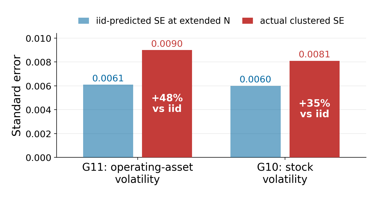
— roughly **51 clusters**, a count fixed by law-adoption geography that added *years* do not
grow. More within-cluster observations do not shrink a clustered SE the way iid N would. The
figure below (`gm_fig_se_vs_n.py`, hard-coding the Phase-3.5 SEs from the findings ledger)
compares the SE an iid model predicts at the extended N against the actual clustered SE:
```{python}
#| eval: true
#| echo: true
import contextlib, io
sys.path.insert(0, "code")
import gm_fig_se_vs_n
with contextlib.redirect_stdout(io.StringIO()):
    gm_fig_se_vs_n.main()   # numbers from gm-cornerstone-findings.md, Phase 3.5
from IPython.display import Image
Image("outputs/figures/gm_se_vs_n.png")
```
For operating-asset volatility the SE *rose* from 0.0078 to 0.0090 on +65% N; an iid model
predicts ≈0.0061 at the extended N, so the actual clustered SE is **+48% above iid**. Stock
volatility shows the same pattern (predicted ≈0.0060, actual 0.0081, **+35% above iid**), but
its larger effect clears the bar anyway. The lesson for students: **more observations do not
buy precision when the thing you cluster on is fixed.** This is an inference-precision limit,
not small-N, and it ties straight back to §5's clustering decision.
## 17. The card we wrote before we ran anything
Every expectation in the scorecard below was frozen *before the first line of estimation code
ran* (`gm-cornerstone-expectations.md`); the verdicts were filled in afterwards. The previous
sections are this card being scored. Two rows are verdicts on the replication process itself,
not on the paper — and they are kept red, not laundered.
| Leg | Written before the code | Found | Verdict |
|---|---|---|---|
| Ln(cash) headline | ≈ +0.121, t ≥ 2 | +0.108, t 2.89 | PASS |
| Cash ratio che/at | ≈ +0.0023, ns | −0.0024, t −0.90 | PASS (null) |
| Event-study leads | flat, all \|t\| < 1.65 | −1.64, −1.45, −1.00, −1.26 | PASS |
| Dynamic phase-in | rises and stabilises | immediate + persistent, dip at k2 | **CHECK** |
| Placebo, three years early | insignificant | +0.0591, t 1.68 | PASS (borderline) |
| Sun–Abraham ATT | sign preserved | +0.101 Python / +0.169 R, both sig. | PASS |
| Delaware excluded | positive, ideally significant | +0.1429, t 2.14 | PASS |
| Cash-flow volatility | ≈ −0.0028, ns | −0.0015, t −0.92 | PASS (null) |
| Stock volatility | ≈ −0.023, t ≤ −2 | −0.0232, t −2.88 | PASS |
| Operating-asset volatility | ≈ −0.015, t ≤ −2 | −0.0152, t −1.69 | **CHECK** |
| *Phase-3 reading:* vol coefficients scale down with the lower vol levels | (written after Phase 3, not before) | level gap widened while the coefficient rose to GM's | **RETRACTED** |
| *Conjecture:* the soft leg just needs more N | iid scaling put t ≈ −2.1 at GM's N | N reached, t stayed −1.69, SE 48% above iid | **REFUTED** |
The reason the green rows mean anything is that the middle column was frozen before any code
ran: a PASS you could not have failed is not a pass. The two red rows are the honest part — a
reading withdrawn (§15's level caveat) and a conjecture the data refuted (§16's clustering
finding). Card: `gm-cornerstone-expectations.md`; the two red rows: `gm-cornerstone-findings.md`,
Phase 3.5.
## 18. What to believe, and how much
The deliverable of the whole segment is not any single coefficient; it is an ordering of the
claims by how much weight each carries.
1. **Insulated managers hold more cash — solid.** The headline (+0.108, t 2.89) survived four
attempted breakages: the event study, the placebo, the Sun–Abraham re-estimation, and the
drop-Delaware-plus-leave-one-out sweep. Nothing moved the sign, and little moved the
magnitude.
2. **Equity risk falls — reproduces.** Stock volatility declines at t −2.88 on a daily panel
assembled from Compustat with no CRSP — the harder road, and the one students can imagine
walking.
3. **Business risk falls — directional only.** Operating-asset volatility lands on GM's
magnitude but at t −1.69, and §16 explained why more data will not fix it. This is the
honest weak point of the risk story.
4. **Cash-flow volatility is unchanged — a null, and GM's own.** Reported as a result because
reproducing the paper's null *is* the result.
Then the hand-off to Part 2: today the danger was a variable wrongly included or wrongly
omitted in a *causal* design. Next it is the same disease in an *asset-pricing* model — where
what gets left out of the specification prices what stays in.
## 19. Skeptic's appendix
Four objections a careful reader would raise, each already measured, plus two things
genuinely out of reach.
1. **Parallel trends holds by the bar, not pristinely.** The event-study leads are all mildly
negative and $k=-5$ sits at t −1.64; the three-years-early placebo is +0.0591 (t 1.68).
Both clear their thresholds and both lean the same soft way (`gm-cornerstone-findings.md`,
caveat 2). Reported, not hidden.
2. **Delaware dominance.** 53% of observations on the baseline panel, 55.8% extended, adopting
in 1988, with the never-treated share only 11% (9% extended). Answered by §13's drop-DE and
leave-one-out sweeps, but the caveat stays live.
3. **Our volatility levels run below GM's.** Stock-vol mean 0.500 against 0.611, op-asset 0.296
against 0.400, cash-flow vol 0.0645 against 0.084 — so the numbers in §15 are read
percent-of-mean, where −0.0232 is 4.6% of our mean against GM's 4.3% of pre-law
(`gm-stock-vol-2026.md`, sample block). The "proportional down-scaling" reading was retracted.
4. **Incorporation is the current Compustat header**, not Cohen (2012) historical coding.
Gormley–Matsa footnote 6 settles it: historical coding changes treatment status for about
2% of observations, conclusions unchanged, so this build is their stated robustness variant.
Genuinely out of reach, and worth one honest sentence each if asked: **performance-related
exit** (Gormley–Matsa build it from CRSP delisting codes 400–500, 550, 552, 560, 561, 572,
574, 580, 584 — "we use CRSP delisting codes to construct an indicator variable that equals
one when firms exit our sample because of bankruptcy, liquidation, or other performance-related
reasons" — which we do not have), and the **literal Table-7 acquisitions outcome** (Table A.2:
"Number of acquisitions Calculated using the Securities Data Company (SDC) …", which is
licence-gated).
Two further conjectures are flagged and deliberately *not* asserted, because neither was
measured here: that the extended window spans more volatility-regime heterogeneity (2008, 2020),
and that Compustat-`secd` daily returns are noisier than CRSP (untestable — CRSP is not on
disk). Neither belongs on a slide as an explanation.
## Sources
- Gormley, T. A., & Matsa, D. A. (2016). *Playing it safe? Managerial preferences, risk, and
agency conflicts.* Journal of Financial Economics 122(3), 431–455. All GM quotes above are
verbatim from the paper's Sections 3–4 and Appendix Table A.2.
- Bertrand, M., & Mullainathan, S. (2003). *Enjoying the quiet life? Corporate governance and
managerial preferences.* Journal of Political Economy 111(5) — the 30-state BC-law dating GM
builds on.
- Pinnell, C. (2000). *State Takeover Laws* — the source for GM's three additional states
(Iowa, Oregon, Texas).
- Gormley, T. A., & Matsa, D. A. (2014). *Common errors: How to (and not to) control for
unobserved heterogeneity.* Review of Financial Studies 27(2), 617–661 — the AvgE
"common error" doctrine behind §14.
- Sun, L., & Abraham, S. (2021). *Estimating dynamic treatment effects in event studies with
heterogeneous treatment effects.* Journal of Econometrics — the §12 estimator.
- Angrist, J. D., & Pischke, J.-S. *Mostly Harmless Econometrics* — the bad-controls warning of §14.
- Build provenance: the committed scripts `code/gm_*.py`, `gm_did_rcheck.R`,
`gm_phase3_rcheck.R`, and the frozen result ledgers `outputs/gm-*.md`.
## Session info
The free spine of this document ran under the versions below; the quoted econometrics ran under
`pyfixest`, cross-checked in R `fixest` per `gm_did_rcheck.R` / `gm_phase3_rcheck.R`.
```{python}
#| eval: true
#| echo: true
import sys, platform, pandas, matplotlib
sys.path.insert(0, "code")
import gm_bc_dates as bc

print("Python     :", platform.python_version())
print("pandas     :", pandas.__version__)
print("matplotlib :", matplotlib.__version__)
print("gm_bc_dates:", len(bc.BC_LAWS), "states,",
      len(bc.bm_only()), "in the BM-only subset")
print("econometrics quoted from ledgers; ran under pyfixest, cross-checked in R fixest")
```