| Before | After | Change | |
|---|---|---|---|
| New Jersey (treated) | 20.44 | 21.03 | 0.59 |
| Pennsylvania (comparison) | 23.33 | 21.17 | -2.17 |
Empirical Economics
Lecture 6: Difference-in-differences
Outline
Course Overview
- Linear Model I
- Linear Model II
- Time Series and Prediction
- Panel Data I
- Panel Data II
- Difference-in-differences
- Track-specific applications
What do we do today?
We investigate one question throughout the lecture:
Did New Jersey’s 1992 minimum-wage increase reduce employment at fast-food restaurants?
Card and Krueger surveyed restaurants in New Jersey, where the minimum wage rose from $4.25 to $5.05, and in neighboring Pennsylvania, where it did not. Their design shows how a credible comparison group can supply a missing counterfactual.
What should you be able to do?
By the end of the lecture, you should be able to:
- calculate and interpret a \(2\times2\) difference-in-differences estimate;
- state the counterfactual encoded by parallel trends, and explain why it depends on the scale of the outcome;
- explain why pre-treatment evidence supports, but cannot prove, identification;
- interpret the interaction coefficient and choose an inference strategy; and
- recognize when staggered adoption makes conventional two-way fixed effects problematic, and name an estimator that repairs it.
What do you predict?
New Jersey raised its minimum wage in April 1992. Standard competitive theory predicts that a binding wage floor reduces employers’ demand for labor.
Commit to a prediction
Compared with similar restaurants in Pennsylvania, what happened to employment in New Jersey?
- It fell.
- It was unchanged.
- It rose.
Write down both your prediction and the comparison you would use to evaluate it.
One policy, four means
The design is a border, not a laboratory
New Jersey’s minimum wage rose from $4.25 to $5.05 on 1 April 1992. Card and Krueger telephoned 410 Burger King, KFC, Wendy’s and Roy Rogers outlets in February–March and again in November–December 1992: 331 in New Jersey and 79 in eastern Pennsylvania.
Three design choices do the work. The outcome is measured identically in both states. The comparison restaurants sit across a state line, in the same regional labour market. And each restaurant is observed twice, so each supplies its own change.
Why fast food?
The industry employs many minimum-wage workers, product and hiring practices are standardised within chains, and employment is easy to define. The setting was chosen so that a simple comparison would be informative.
Neither post-policy level identifies the effect
After the increase, New Jersey restaurants employed an average of 21.03 full-time-equivalent workers, compared with 21.17 in Pennsylvania.
That -0.14 difference does not by itself measure the policy effect. The two states may have differed before the policy, and those baseline differences may also influence employment.
The causal question
What would employment at New Jersey restaurants have been after April 1992 if New Jersey had not raised its minimum wage?
Two simple comparisons, two strong assumptions
Two single differences are available, and each rests on an assumption we have no reason to believe.
The cross-sectional comparison, New Jersey versus Pennsylvania after the policy, assumes the two states would have had the same employment level without it. The before-and-after comparison, New Jersey in November versus New Jersey in February, assumes nothing else changed in New Jersey over those nine months.
What DiD buys
Differencing across states removes anything that is fixed within a state. Differencing across time removes anything common to both states. DiD needs neither assumption above; it needs the weaker claim that the two would have moved together.
The four observed means reveal two changes
New Jersey started lower, so comparing post-policy levels ignores a pre-existing gap. Comparing New Jersey before and after is also insufficient: employment may have changed over time even without the policy.
DiD uses Pennsylvania’s change to estimate that untreated time trend.
Can you recover the difference-in-differences?
Retrieval prompt
Using the four means, calculate:
- the change in New Jersey;
- the change in Pennsylvania; and
- the difference between those changes.
What does the sign of your answer say about the prediction you made?
New Jersey employment rose by 2.75 FTE relative to Pennsylvania
\[ \begin{aligned} \widehat{\Delta}_{NJ} &= 21.03-20.44=0.59,\\ \widehat{\Delta}_{PA} &= 21.17-23.33=-2.17,\\ \widehat{\tau}_{DiD} &= \widehat{\Delta}_{NJ} -\widehat{\Delta}_{PA}=2.75. \end{aligned} \]
The estimate is about 13.5% of New Jersey’s pre-policy mean. It contradicts the prediction that employment fell relative to Pennsylvania. Whether it is causal depends on the comparison group’s credibility.
DiD constructs the missing New Jersey counterfactual
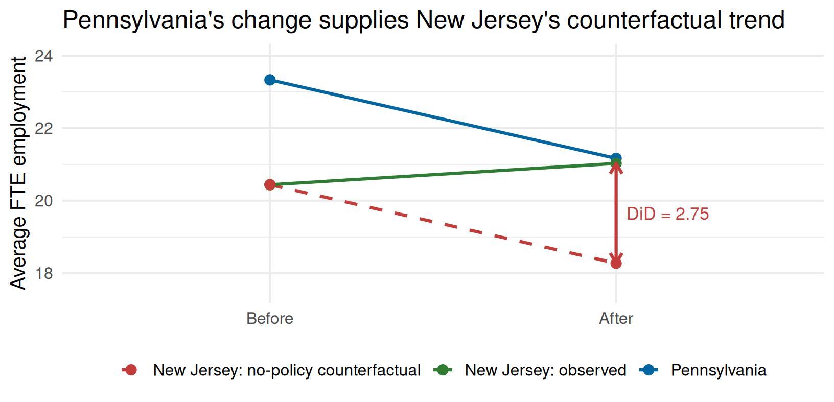
The dashed endpoint is not observed. It equals New Jersey’s initial level plus Pennsylvania’s change: 18.27. The vertical distance from there to the observed 21.03 is the DiD estimate.
What makes the comparison causal?
Potential outcomes name the missing quantity
Let \(D_i=1\) denote a New Jersey restaurant and \(D_i=0\) a Pennsylvania restaurant. Let \(t=0\) be before and \(t=1\) after the increase.
\(Y_{it}(1)\) is restaurant \(i\)’s employment at time \(t\) under the higher minimum wage; \(Y_{it}(0)\) is its employment without that policy. The target is the average treatment effect on the treated:
Estimand: ATT
\[ ATT=E\!\left[Y_{i1}(1)-Y_{i1}(0)\mid D_i=1\right]. \]
We observe \(Y_{i1}(1)\) for New Jersey. The missing term is \(E[Y_{i1}(0)\mid D_i=1]\): post-policy New Jersey employment without the increase.
Four assumptions connect the observed data to the ATT
Identification conditions
Consistency: observed employment equals the potential outcome under the policy actually received.
No anticipation: before April, New Jersey outcomes are untreated outcomes: \(Y_{i0}=Y_{i0}(0)\).
No interference: New Jersey’s policy does not change Pennsylvania restaurants’ outcomes, and one restaurant’s exposure does not alter another’s.
Parallel trends: without the policy, average employment would have changed by the same amount in both states: \[ E[Y_{i1}(0)-Y_{i0}(0)\mid D_i=1] =E[Y_{i1}(0)-Y_{i0}(0)\mid D_i=0]. \]
The assumptions are claims about the setting, not mechanical properties of the estimator.
Parallel trends is about changes, not levels
New Jersey and Pennsylvania need not begin with equal employment. They may differ permanently in restaurant size or composition.
Parallel trends instead says that the average untreated change in Pennsylvania represents the unobserved average untreated change in New Jersey. It therefore converts an observed trend into a counterfactual:
\[ \underbrace{E[Y_{i1}(0)\mid D_i=1]}_{\text{missing NJ post outcome}} = \underbrace{E[Y_{i0}(0)\mid D_i=1]}_{\text{NJ before}} + \underbrace{E[Y_{i1}(0)-Y_{i0}(0)\mid D_i=0]}_{\text{PA change}}. \]
Why does the population DiD identify the ATT?
Write the observed change as \(\Delta Y_i=Y_{i1}-Y_{i0}\). Then
\[ \tau_{DiD} = \underbrace{E[\Delta Y_i\mid D_i=1]}_{\text{change in New Jersey}} - \underbrace{E[\Delta Y_i\mid D_i=0]}_{\text{change in Pennsylvania}}. \]
Consistency and no anticipation give the first line below. Parallel trends then replaces Pennsylvania’s untreated change with New Jersey’s:
\[ \begin{aligned} \tau_{DiD} &=E[Y_{i1}(1)-Y_{i0}(0)\mid D_i=1] -\underbrace{E[Y_{i1}(0)-Y_{i0}(0)\mid D_i=0]}_{\text{PA untreated change}}\\ &=E[Y_{i1}(1)-Y_{i0}(0)\mid D_i=1] -\underbrace{E[Y_{i1}(0)-Y_{i0}(0)\mid D_i=1]}_{\text{NJ untreated change}}\\ &=E[Y_{i1}(1)-Y_{i1}(0)\mid D_i=1] =ATT. \end{aligned} \]
Four sample means estimate the population contrast
The population contrast \(\tau_{DiD}\) is an estimand. Its sample analogue is the estimator
\[ \widehat{\tau}_{DiD} = (\bar Y_{NJ,after}-\bar Y_{NJ,before}) - (\bar Y_{PA,after}-\bar Y_{PA,before}). \]
Sampling variation means \(\widehat{\tau}_{DiD}\) need not equal \(\tau_{DiD}\) in a particular sample. In Card and Krueger’s data, \(\widehat{\tau}_{DiD}=2.75\) FTE workers.
Interpretation with assumptions attached
If consistency, no anticipation, no interference, and parallel trends hold, the sample DiD estimates the ATT for New Jersey restaurants.
Parallel trends is not scale-free
Parallel trends in levels and parallel trends in logs are different assumptions. They coincide only in knife-edge cases, when the untreated change is zero, or when the two groups start from the same level. Otherwise groups cannot grow by the same number of jobs and by the same percentage.
| Outcome | DiD estimate | Std. error | t |
|---|---|---|---|
| Employment (FTE) | 2.722 | 1.335 | 2.038 |
| Log employment | 0.078 | 0.049 | 1.598 |
Both estimates are positive, but only the level specification clears the conventional significance threshold. (Both use the 378 restaurants with positive employment in both waves, so the level estimate differs slightly from 2.75.) The scale is part of the assumption: choose it substantively, before seeing results.
Which assumption does each scenario threaten?
Retrieval prompt
Match each scenario to the most direct threat.
- Restaurants raise wages and alter hiring before April.
- Pennsylvania restaurants lose customers to New Jersey restaurants.
- A New Jersey tax credit begins in April and raises restaurant employment.
- A restaurant is coded as treated even though it was exempt from the wage increase.
Use: no anticipation, no interference, parallel trends, or consistency.
The matches are 1: no anticipation; 2: no interference; 3: parallel trends; 4: consistency. In applications, one event can threaten more than one condition, so institutional knowledge matters.
The same contrast in a regression
One interaction coefficient reproduces the four-mean DiD
Estimate
\[ Y_{it}=\beta_0+\beta_1D_i+\beta_2Post_t +\beta_3(D_i\times Post_t)+u_{it}. \]
\(\beta_0\) is Pennsylvania’s pre-policy mean; \(\beta_1\) is New Jersey’s pre-policy level difference; and \(\beta_2\) is Pennsylvania’s change. The interaction \(\beta_3\) is New Jersey’s additional change:
\[ \beta_3=(\bar Y_{NJ,after}-\bar Y_{NJ,before}) -(\bar Y_{PA,after}-\bar Y_{PA,before}). \]
Thus OLS and the hand calculation are numerically identical in the saturated \(2\times2\) design.
The interaction returns the same 2.75 FTE estimate
Card–Krueger result
\[\widehat{\beta}_3=\widehat{\tau}_{DiD}=2.75\text{ FTE workers} \qquad(\text{s.e. }1.31,\ 13.5\%\text{ of the pre-policy mean}).\]
Code
coeftable(feols(employment ~ treated * time,
                data = card_krueger_data, cluster = ~sheet))
##                        Estimate Std. Error   t value     Pr(>|t|)
## (Intercept)           23.331169   1.346540 17.326755 8.357742e-51
## treatedTRUE           -2.891761   1.436604 -2.012914 4.478013e-02
## timeAfter             -2.165584   1.218028 -1.777943 7.615801e-02
## treatedTRUE:timeAfter  2.753606   1.306485  2.107645 3.567124e-02
## attr(,"vcov_type")
## [1] "Clustered (sheet)"
The regression buys convenience, not credibility: the coefficient becomes causal only under the identification assumptions.
DiD is the two-way fixed-effects model of Lectures 4 and 5
The interaction model has an equivalent panel form. Replace the group and period dummies with unit and time fixed effects, and let \(W_{it}=D_i\times Post_t\) indicate that unit \(i\) is treated at time \(t\):
\[ Y_{it}=\alpha_i+\lambda_t+\delta W_{it}+u_{it}. \]
With two groups and two periods, \(\widehat\delta=\widehat\beta_3\) exactly. The fixed effects do what differencing did: \(\alpha_i\) absorbs everything permanent about a restaurant, \(\lambda_t\) everything common to the period.
One model, two readings
Everything you learned about within variation and clustering in Lectures 4 and 5 applies here. What is new is not the estimator but the design: which units are compared, and why their untreated paths should agree.
Panel or repeated cross-sections?
DiD does not require the same units twice. It requires a treated and a comparison group observed before and after, and the four means can come from independent samples, a labour force survey, for example.
With a panel, the composition of each group is held fixed and each unit supplies its own change. With repeated cross-sections, a shift in who is sampled can move a group mean without moving any individual outcome.
Composition is an identification problem
Attrition makes a panel behave like a repeated cross-section. Card and Krueger’s balanced first differences give \(2.75\), close to the 2.75 from the pooled means: reassuring, but something to check rather than assume.
Regression does not automatically solve inference
Repeated outcomes for the same restaurants are correlated, while every restaurant in a state receives the same policy exposure. IID standard errors treat those observations as more independent than they are.
Cluster where treatment is assigned
In DiD, cluster standard errors at the level at which treatment varies when there are enough independent clusters. With many treated and comparison states, that commonly means clustering by state.
Card and Krueger have only two state-level clusters. Conventional cluster-robust state-level standard errors are therefore not credible. The 2.75 estimate remains a descriptive DiD contrast, but reliable inference needs more assignment units or a design-based argument.
Serial correlation inflates DiD \(t\)-statistics
Bertrand, Duflo and Mullainathan (2004) assigned placebo laws to random states in real wage data, where the true effect is zero by construction. With conventional standard errors, the placebo “effect” was significant at the 5% level in up to 45% of the runs.
The reason is that outcomes such as state employment or wages are highly persistent. Many periods of a serially correlated series carry far less information than the sample size suggests.
More periods are not more information
Adding years to a DiD panel shrinks conventional standard errors mechanically, but the additional years contain much the same shock. Cluster on the unit of assignment, or collapse the panel to one pre- and one post-period per unit and difference.
What to do when clusters are few
The cluster-robust variance estimator needs many clusters, not many observations. With a handful of treated units, three practical routes remain.
Collapse and difference: reduce each unit to one pre and one post mean, so that serial correlation cannot accumulate. Wild cluster bootstrap: resample cluster-level residual signs, which performs far better than the asymptotic formula for five to thirty clusters. Randomization inference: reassign the placebo treatment across units and ask where the actual estimate falls in that distribution.
Retrieval prompt
Twelve states adopt a policy, thirty-eight do not, and you have twenty years of annual data. What is your cluster, and how many are there?
Covariates change the identifying assumption
With pre-treatment covariates \(X_i\), a model can target conditional parallel trends:
\[ E[Y_{i1}(0)-Y_{i0}(0)\mid D_i=1,X_i] =E[Y_{i1}(0)-Y_{i0}(0)\mid D_i=0,X_i]. \]
Covariates can improve precision or make treated and comparison units more comparable when that conditional claim is substantively credible. Useful examples include restaurant chain and other characteristics fixed before the policy.
Do not control for consequences of treatment
A variable measured after treatment may itself respond to the minimum wage. Conditioning on such a “bad control”, for example, post-policy staffing composition, can introduce bias rather than remove it.
Not every New Jersey restaurant was equally treated
A binary treatment indicator hides something the data know. About 9% of New Jersey restaurants already paid at least $5.05 before April, so the new floor did not bind for them. For a restaurant paying the old $4.25 minimum, it required a wage increase of almost 19%.
Card and Krueger therefore define an intensity measure,
\[ GAP_i=\frac{5.05-W_{i,\text{before}}}{W_{i,\text{before}}} \quad\text{if it is positive, and }0\text{ otherwise,} \]
which is zero for every Pennsylvania restaurant and for unaffected New Jersey restaurants.
Intensity turns one contrast into a dose-response
Regress each restaurant’s employment change on its gap:
| Specification | Coefficient on GAP | Std. error |
|---|---|---|
| Gap only | 12.49 | 6.02 |
| Gap, chain and ownership controls | 11.92 | 6.21 |
Moving from an unaffected restaurant to one facing the full 18.8% increase implies about \(2.35\) additional FTE workers: the same positive sign as the \(2\times2\).
Why this is a stronger design
The comparison now runs within New Jersey as well as across the border, so any shock common to the whole state is differenced out.
Your prediction, revisited
Neither design finds the predicted employment loss. Both find a small positive estimate: 2.75 FTE across the border, and a positive dose-response within New Jersey.
The honest reading is not “minimum wages raise employment”. It is that in this labour market, at this size of increase, a large negative effect is inconsistent with the data, while the confidence intervals still admit modest effects of either sign.
What would change your mind?
Which single piece of additional evidence would most move you: a longer pre-treatment series, more states, or a different measure of employment?
The same design, different data, different answer
Neumark and Wascher (2000) re-examined the question with payroll records rather than telephone interviews for a subset of the same restaurants, and reported an employment decline. Card and Krueger (2000) replied using administrative unemployment-insurance data for the whole industry, and again found no decline.
Both sides used the same New Jersey–Pennsylvania comparison, so the dispute was mostly about measurement, though the payroll sample was itself assembled non-randomly, which is part of what was contested.
Two separate problems
A design tells you which comparison identifies the effect. It does not tell you whether the outcome is measured well. Report how the outcome is constructed, and check whether the result survives an alternative source.
Trends before treatment
Pre-treatment data make parallel trends more credible
Parallel trends is a claim about the unobserved post-treatment counterfactual, so it cannot be tested directly. With several pre-treatment periods we can ask a related question: did the two groups move together before treatment?
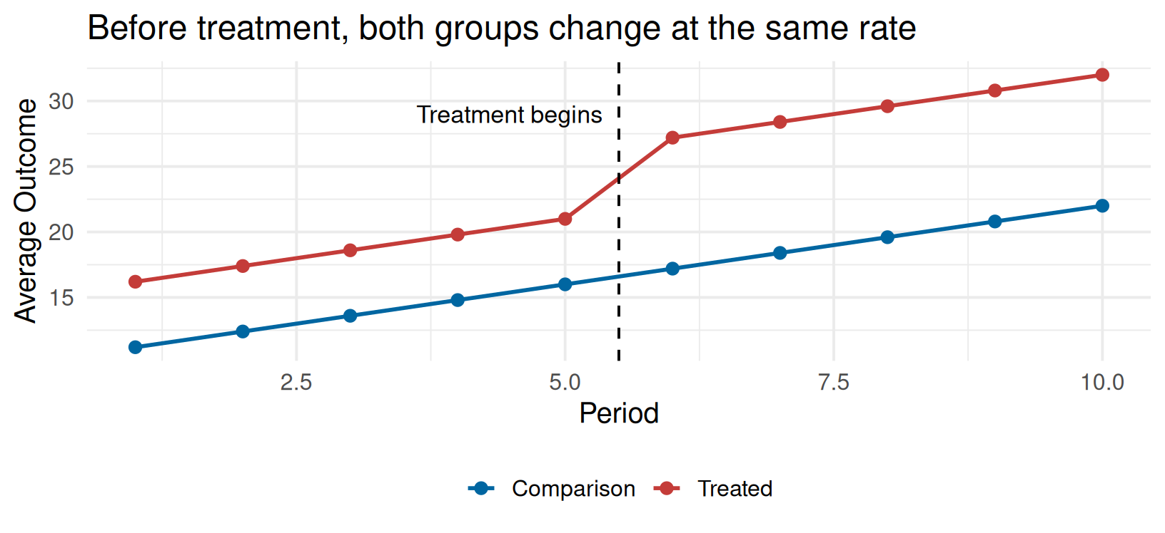
What the graph can establish
Similar pre-treatment paths support the design, but do not prove it. A shock that hits only the treated group when treatment begins still invalidates the post-treatment counterfactual.
Lead coefficients are diagnostics, not a verdict
With common treatment timing, interact the treated-group indicator with relative-time indicators. Omit one pre-treatment period, usually \(k=-1\), as the reference:
\[ y_{it} = \alpha_i + \lambda_t + \sum_{\substack{k=-K \\ k\neq -1}}^{L} \delta_k D_{it}^k + u_{it} \]
Here \(D_{it}^k\) equals one for a treated unit observed \(k\) periods from treatment. Each lead \(\delta_k\) for \(k<-1\) estimates a relative pre-treatment difference compared with \(k=-1\).
Do not interpret ‘insignificant’ as ‘parallel’
Failure to reject the leads may simply reflect imprecise estimates. Inspect their confidence intervals and economic magnitudes, consider a joint test, and explain why the comparison group is credible. Even precisely estimated zero leads cannot rule out a confounding shock that starts with treatment.
What would the pre-treatment evidence tell you?
Retrieval prompt
Suppose every lead is statistically insignificant, but its 95% confidence interval includes effects between \(-8\) and \(+8\) jobs. Can you conclude that parallel trends is plausible?
No. The data are also consistent with economically important differential trends. “No statistically significant difference” is not evidence that the difference is small.
Stronger support combines reasonably precise leads near zero, similar responses to earlier shocks, a defensible comparison group, and no other event that begins with treatment.
Pre-testing changes the estimate you report
Running a pre-trends test and continuing only when it passes is itself a selection rule. Roth (2022) shows that conditioning on passing a low-powered test keeps the samples in which noise happened to flatten the leads, which biases the surviving estimates and distorts their coverage.
The constructive response is to replace the test with a sensitivity analysis. Rambachan and Roth (2023) ask a different question: how large would a differential trend have to be, relative to the pre-treatment variation we can see, before the conclusion changes?
A more useful sentence
“The estimate remains positive unless the post-treatment differential trend is more than twice the largest pre-treatment deviation” says more than “the pre-trends test does not reject.”
Effects over time
Relative-time coefficients reveal dynamics
The two-period DiD coefficient averages everything after treatment into one number. With several periods, a dynamic DiD (often called a panel event study) asks whether an effect appears immediately, grows, fades, or reverses.
For common treatment timing, the same model used for lead diagnostics also provides post-treatment estimates:
\[ y_{it} = \alpha_i + \lambda_t + \sum_{\substack{k=-K \\ k\neq -1}}^{L} \delta_k D_{it}^k + u_{it}. \]
\(\alpha_i\) absorbs permanent unit differences and \(\lambda_t\) absorbs common calendar-time shocks. Under the DiD assumptions, \(\delta_k\) for \(k\geq0\) is the treatment effect at event time \(k\), relative to \(k=-1\).
Normalization
\(\delta_{-1}=0\) by construction; it was not estimated to be zero. Cluster standard errors at the level where treatment is assigned when the number of clusters permits credible cluster-based inference.
A world where we know the answer
To see what the estimator recovers, we build a world in which the truth is chosen rather than estimated. Half of 200 units are treated in period 7. The true effect is \(1.2\) on impact, rises to \(2.5\), and then stays there; every unit also has its own level and shares a common time trend.
Code
event_sim <- expand.grid(id = 1:200, t = 1:12) |>
  mutate(
    treated = id <= 100,
    k = t - 7,
    effect = if_else(treated & k >= 0, true_path[pmin(pmax(k, 0), 5) + 1], 0)
  ) |>
  group_by(id) |>
  mutate(unit_effect = rnorm(1, 0, 3)) |>
  ungroup() |>
  mutate(y = 10 + unit_effect + 0.4 * t + effect + rnorm(n(), 0, 2))

feols(y ~ i(k, treated, ref = -1) | id + t, data = event_sim, cluster = ~id)
Nothing in the estimator knows the true path. If the coefficients trace it out, the design works in this world, which is the only place we can ever check.
Anticipation and dynamics in one picture
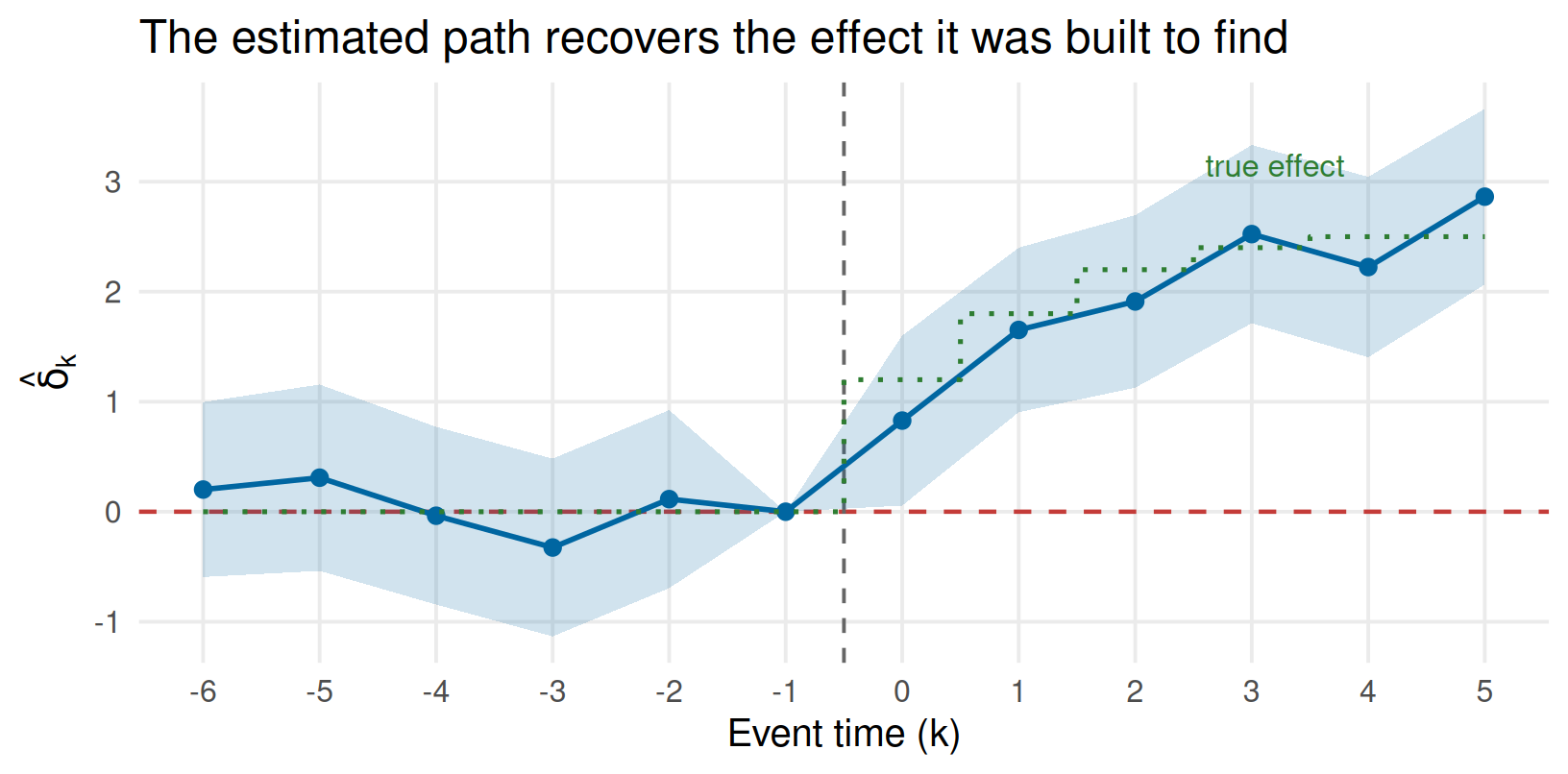
The leads sit near zero, and the post-treatment estimates track the true growth. Confidence intervals widen at the ends, where fewer units contribute.
How to read and report an event study
Report the reference period explicitly, and use the same one everywhere: a plot with \(\delta_{-1}\) silently omitted invites the reader to mistake a normalization for a finding.
At the ends of the window, few units are observed and the estimates are noisy. Bin the extreme leads and lags into a single “\(\le -K\)” and “\(\ge L\)” category rather than reporting a long tail of imprecise coefficients, and say how many units contribute at each event time.
A shape is not a mechanism
An effect that fades may mean adjustment, or it may mean that the comparison group is catching up for reasons unrelated to the policy. The event-study plot constrains the story; it does not supply one.
Staggered adoption
Different treatment dates create different cohorts
Suppose some units adopt in 2023, others in 2025, and some never adopt. Let \(G_i\) denote unit \(i\)’s first treatment period. Units with the same \(G_i=g\) form treatment cohort \(g\).
| Group | 2022 | 2023 | 2024 | 2025 |
|---|---|---|---|---|
| Cohort \(g=2023\) | Untreated | Treated | Treated | Treated |
| Cohort \(g=2025\) | Untreated | Untreated | Untreated | Treated |
| Never treated | Untreated | Untreated | Untreated | Untreated |
In 2023 and 2024, the 2025 cohort is not yet treated and can help form a counterfactual for the 2023 cohort. Once treated, it can no longer serve that role.
Conventional TWFE can mix credible and contaminated comparisons
A single two-way fixed-effects event-study regression looks familiar, but with staggered timing its coefficients need not recover a simple average of causal effects.
The regression can use an already-treated cohort as a comparison for a newly treated cohort. If effects vary across cohorts or over time, the outcome of the “control” cohort already contains treatment effects.
A regression coefficient is not a comparison-group argument
Before interpreting a staggered-adoption estimate, identify which untreated observations supply each cohort’s counterfactual. Conventional TWFE does not guarantee that only never-treated or not-yet-treated units are used.
TWFE averages every \(2\times2\), including the forbidden ones
Goodman-Bacon (2021) shows that the static TWFE coefficient is a weighted average of all possible \(2\times2\) DiD comparisons in the panel, with weights determined by group sizes and by treatment-timing variance.
Three kinds of comparison appear:
- an early cohort against the never-treated – clean;
- an early cohort against a not-yet-treated later cohort – clean;
- a later cohort against an already-treated earlier cohort – forbidden.
In the third comparison the “control” group’s outcome is already changing because of its own treatment. If effects grow with exposure, that change enters the estimate with a negative sign.
A simulation where TWFE misses almost everything
Two cohorts adopt, in periods 5 and 12, sixty units never adopt, and every treated unit’s effect grows by \(0.5\) for each period of exposure. Every individual treatment effect is positive.
| Quantity | Estimate |
|---|---|
| True ATT (known by construction) | 3.62 |
| Static TWFE coefficient | 0.79 |
| Sun–Abraham aggregate ATT | 3.53 |
TWFE recovers about 22% of the true effect, because the long-treated early cohort keeps being used as a control for the later one. The cohort-robust estimator, which never makes that comparison, is close to the truth.
Cohort-time effects keep the comparisons explicit
Estimate a separate effect for cohort \(g\) in calendar period \(t\):
\[ ATT(g,t)=E\!\left[Y_{it}(1)-Y_{it}(0)\mid G_i=g\right]. \]
Under no anticipation and a suitable cohort-specific parallel-trends assumption, compare cohort \(g\)’s change from its last untreated period \(g-1\) with the same change among units untreated through \(t\):
\[ \widehat{ATT}(g,t) =\Delta\bar Y_{g,t} -\Delta\bar Y_{\mathcal C(g,t),t}. \]
\(\mathcal C(g,t)\) should contain never-treated or not-yet-treated units, not units already exposed to treatment. Modern group-time DiD estimators construct these comparisons first and then aggregate them across cohorts or event times.
A menu of cohort-robust estimators
| Estimator | Comparison group | Aggregation |
|---|---|---|
| Callaway–Sant’Anna (2021) | never- or not-yet-treated | \(ATT(g,t)\), then weight |
| Sun–Abraham (2021) | last-treated or never-treated | interaction-weighted event study |
| Borusyak–Jaravel–Spiess (2024) | all untreated observations | impute \(Y_{it}(0)\), then average |
| de Chaisemartin–D’Haultfœuille (2020) | not-yet-treated switchers | period-by-period switchers |
They differ in which untreated observations they use and how they aggregate, not in what they are trying to avoid.
What they share
Each builds only clean comparisons first and aggregates second. With a single treatment date and no effect heterogeneity, they all collapse back to the familiar TWFE estimate.
Report effects only where untreated comparisons exist
Return to the adoption table. For the 2023 cohort:
- In 2023 and 2024, use the never-treated group and the not-yet-treated 2025 cohort.
- In 2025, the 2025 cohort is treated, so only the never-treated group remains available.
- If there is no never-treated group, the 2023 cohort has no clean contemporaneous comparison in 2025.
Support determines the estimand
Do not report a long event-time horizon merely because software returns it. Show how many cohorts and untreated comparison units support each estimate, and restrict the window when support disappears.
Can every cohort identify every event-time effect?
Retrieval prompt
All units are treated by 2025, and none is never treated. Can we identify the effect on the 2023 cohort in 2025 using a clean not-yet-treated comparison? What comparison might conventional TWFE use instead?
No. By 2025 no untreated unit remains. Conventional TWFE may still compare the 2023 cohort with units treated in 2025, or compare newly treated units with the already-treated 2023 cohort. Both comparisons involve treated outcomes and require additional restrictions to be causal.
If every unit is treated in the same calendar period, event time merely relabels calendar time; event-time dummies are collinear with time fixed effects. See the mathematical explanation.
Threats to credibility
Selection before treatment can mimic an effect
In Ashenfelter’s dip, outcomes fall shortly before units enter treatment. Earnings may drop because of job loss just before participation in a training program, then recover even without training.
Comparing the dip with the post-treatment period exaggerates the program’s effect. Longer pre-treatment histories can reveal this pattern, but choosing a credible comparison group and explaining treatment timing remain essential.
The identifying threat
Treatment is triggered by unusual outcome dynamics, so the treated group’s untreated path may not have followed the control group’s path.
Anticipation contaminates the pre-period
If units change behavior because they know treatment is coming, the observed pre-treatment outcome is no longer an untreated baseline. A firm that slows hiring before a minimum-wage increase illustrates the problem.
Researchers should investigate announcement and implementation dates, redefine event time when appropriate, and avoid using plausibly affected periods as untreated observations.
No anticipation
Before treatment starts, observed outcomes should equal the relevant untreated potential outcomes.
Spillovers contaminate the comparison group
A valid comparison group must remain untreated by both the policy and its indirect effects. If a job fair draws workers away from a neighboring control city, that city’s outcome no longer represents the treated city’s untreated counterfactual.
Spillovers can operate through labor markets, prices, migration, or strategic responses. Redesigning the comparison set or estimating exposure effects is preferable to simply adding controls.
No interference
One unit’s treatment should not change another unit’s potential outcomes unless the design explicitly models that exposure.
A third difference can absorb a common shock
When the comparison group is contaminated by something that also hits the treated group, a triple difference adds a dimension along which only the treated group should respond.
If New Jersey’s economy improved in 1992, the state-level comparison is compromised. But high-wage restaurants inside New Jersey were unaffected by the wage floor, so \[ \text{DDD}=\underbrace{\text{DiD}_{\text{low-wage}}}_{\text{NJ vs PA}} -\underbrace{\text{DiD}_{\text{high-wage}}}_{\text{NJ vs PA}} \] differences out any shock common to all New Jersey restaurants.
Weaker, but not assumption-free
DDD requires only that the bias be the same in the two subgroups. That is weaker than two separate parallel-trends assumptions, but it is still an assumption about unobservables.
Basic DiD allows heterogeneous effects
The 2×2 DiD estimand is an average treatment effect on the treated. Individual treatment effects need not all be the same constant. A single coefficient becomes restrictive when it is used to summarize effects across many groups or post-treatment periods, especially if effects evolve over time.
Panel data or repeated cross-sections can support DiD, but neither rescues an implausible comparison group. When no group has a credible parallel trend, the answer is a different design (a synthetic control built from a weighted combination of untreated units, or an intensity measure) not a longer list of controls.
Practice rule
Choose the outcome scale substantively, show treatment dynamics when possible, and never let regression complexity substitute for a counterfactual argument.
Software
The \(2\times2\) and its standard error
Code
library(dplyr)
library(fixest)
library(haven)
library(tidyr)

fastfood <- read_dta(
  "https://empirical-economics.netlify.app/tutorials/datafiles/fastfood.dta"
) |>
  mutate(
    fte = nmgrs + empft + 0.5 * emppt,
    fte2 = nmgrs2 + empft2 + 0.5 * emppt2,
    d_fte = fte2 - fte,
    treated = state == 1
  )

card_krueger_data <- fastfood |>
  select(sheet, state, treated, fte, fte2) |>
  pivot_longer(c(fte, fte2), names_to = "time", values_to = "employment") |>
  mutate(time = factor(time, levels = c("fte", "fte2")))

# The interaction model. Cluster on the unit that is sampled repeatedly;
# with only two states, a state-level cluster is not available here.
feols(employment ~ treated * time, data = card_krueger_data, cluster = ~sheet) |>
  coeftable()

# The identical estimate as a first difference, one row per restaurant.
feols(d_fte ~ treated, data = fastfood, vcov = "hetero") |>
  coeftable()
Code
import pandas as pd
import pyfixest as pf

ck = pd.read_stata(
    "https://empirical-economics.netlify.app/tutorials/datafiles/fastfood.dta"
)
ck["employment_before"] = ck["nmgrs"] + ck["empft"] + 0.5 * ck["emppt"]
ck["employment_after"] = ck["nmgrs2"] + ck["empft2"] + 0.5 * ck["emppt2"]
ck = ck.melt(
    id_vars=["sheet", "state"],
    value_vars=["employment_before", "employment_after"],
    var_name="time",
    value_name="employment",
)
ck["treated"] = ck["state"] == 1
ck["post"] = ck["time"] == "employment_after"
pf.feols("employment ~ treated * post", data=ck, vcov={"CRV1": "sheet"}).tidy()
Both forms give 2.75. The interaction model uses all observations; the first difference uses only restaurants observed twice, which is why the two samples and the standard errors differ slightly.
An event study with common timing
Code
i() and iplot() do the bookkeeping that makes event studies tedious by hand: one indicator per event time, one omitted reference period, and a plot with confidence intervals on the same scale as the coefficients.
Staggered adoption, done two ways
Code
# What NOT to report on its own: the static TWFE coefficient.
feols(y ~ treat | id + t, data = stag_sim, cluster = ~id) |> coeftable()

# Sun and Abraham: sunab() needs the cohort variable and calendar time.
# Never-treated units carry a cohort value outside the sample (here 10000).
sa <- feols(y ~ sunab(g_sunab, t) | id + t, data = stag_sim, cluster = ~id)
summary(sa, agg = "att")
Code
stag = r.stag_sim
stag["rel"] = (stag["t"] - stag["g"]).where(stag["g"] < 1e5, -1).astype(int)

# Gardner's two-stage estimator: fit the fixed effects on untreated
# observations only, then estimate the event study on the residuals.
pf.did2s(
    stag,
    yname="y",
    first_stage="~ 0 | id + t",
    second_stage="~ i(rel, ref=-1)",
    treatment="treat",
    cluster="id",
).tidy().head()
The R did package and the Python differences package implement the Callaway–Sant’Anna group-time estimator directly.
Takeaways
What did we learn?
- DiD estimates a treated group’s missing counterfactual by combining changes over time with differences across groups.
- Under consistency, no anticipation, no interference, and parallel trends, the 2×2 contrast identifies the ATT on the scale you chose.
- The interaction coefficient reproduces the four-means calculation and is the TWFE model of Lectures 4–5; credible standard errors require clustering at the treatment-assignment level, and serially correlated outcomes make naive ones far too small.
- Pre-treatment estimates can challenge but never prove parallel trends; sensitivity analysis says more than a pre-trends test.
- With staggered adoption, TWFE averages in forbidden already-treated comparisons; prefer cohort-time estimators using never- or not-yet-treated units.
Exit questions: identify the argument
- New Jersey employment rises by 0.6 FTE and Pennsylvania employment falls by 2.1 FTE. What is the DiD estimate?
- In one sentence, what counterfactual does parallel trends supply?
- All pre-treatment lead estimates are statistically insignificant. What can you conclude?
Commit before revealing
Write down each answer and the assumption that makes your causal interpretation possible.
Check your answers
- The estimate is \(0.6-(-2.1)=2.7\) FTE.
- It uses the comparison group’s change to infer how the treated group’s outcome would have changed without treatment.
- The estimates provide no detected evidence against parallel trends over those periods. They do not prove the assumption: the test may have low power, and post-treatment counterfactual trends remain unobserved.
Exit questions: diagnose the design
- A neighboring control region changes hiring because workers cross the border after treatment. Which assumption fails?
- Why can a conventional TWFE event study mislead when treatment timing is staggered and effects differ across cohorts or event time?
- A referee reports that your result holds in levels but not in logs. Is one of the two specifications wrong?
Check your answers
- No interference fails: treatment spills into the comparison group.
- TWFE may use already-treated units as controls. Their evolving treatment effects contaminate the comparison.
- Neither is wrong as arithmetic. They encode different parallel-trends assumptions, and at most one of them can hold. Say which one your economics implies, and report the other as a robustness check.
Appendix
Source notes
- Card, D. and A. B. Krueger (1994), “Minimum Wages and Employment: A Case Study of the Fast-Food Industry in New Jersey and Pennsylvania”, American Economic Review 84(4), 772–793. The data file contains 410 restaurants.
- The payroll-data exchange: Neumark, D. and W. Wascher (2000), “Comment”, American Economic Review 90(5), 1362–1396, and Card, D. and A. B. Krueger (2000), “Reply”, 1397–1420.
- Bertrand, M., E. Duflo and S. Mullainathan (2004), “How Much Should We Trust Differences-in-Differences Estimates?”, Quarterly Journal of Economics 119(1), 249–275.
- Goodman-Bacon, A. (2021), Journal of Econometrics 225(2), 254–277; Callaway, B. and P. H. C. Sant’Anna (2021), 200–230; Sun, L. and S. Abraham (2021), 175–199.
- Roth, J. (2022), AER: Insights 4(3), 305–322; Rambachan, A. and J. Roth (2023), Review of Economic Studies 90(5), 2555–2591.
Why the interaction equals the four means
Take expectations of \(Y_{it}=\beta_0+\beta_1D_i+\beta_2Post_t+\beta_3D_iPost_t+u_{it}\) in each of the four cells:
\[ \begin{aligned} E[Y\mid D=0,Post=0]&=\beta_0, & E[Y\mid D=0,Post=1]&=\beta_0+\beta_2,\\ E[Y\mid D=1,Post=0]&=\beta_0+\beta_1, & E[Y\mid D=1,Post=1]&=\beta_0+\beta_1+\beta_2+\beta_3. \end{aligned} \]
Differencing within each group gives \(\beta_2+\beta_3\) for the treated and \(\beta_2\) for the comparison group; differencing again leaves \(\beta_3\).
The model has four parameters and four cell means, so it is saturated: OLS fits the cells exactly, and no functional-form assumption is being imposed. That is why the regression and the hand calculation cannot disagree.
The End

Empirical Economics: Lecture 6 - Difference-in-differences (Finance and Entrepreneurship Tracks)