Solutions Tutorial 3: The Linear Model II

Retrieval practice

1. \(\beta_j\) is the effect of a one-unit change in \(x_j\) with the other included regressors held fixed, and a control is chosen for its causal role: a pre-treatment confounder belongs in the model, a mediator or collider generally does not.
2. \(R_j^2\) is then high, so \(SST_j(1-R_j^2)\) is small and \(\hat\beta_j\) has a large variance: its separate effect is hard to estimate precisely.
3. An \(F\)-test is needed when several restrictions are tested jointly; with a single restriction \(F=t^2\), so the two tests agree.
4. The return to education for women is \(\beta_2+\beta_3\).
5. They change only the estimated standard errors, never the coefficients, and they repair neither omitted-variable bias nor any other identification problem.

Solutions

Reading regression output

1. The lotsize estimate is 0.00207 thousand dollars per square foot. Holding house size and bedrooms constant, one additional square foot of land is associated with about $2.07 more in predicted price. A 1,000-square-foot larger parcel is therefore associated with about $2,068 more.

2. Holding square footage and bedrooms constant, a colonial-style house is estimated to cost about $13,078 more than a non-colonial house. Its \(t\)-statistic is about 0.85 and its \(p\)-value is about 0.399, so we fail to reject \(H_0:\beta_{colonial}=0\) at 5%. The point estimate still has an economic interpretation; the large \(p\)-value says that the sample does not estimate it precisely enough to establish a population difference.

3. No. A larger \(R^2\) means better in-sample fit. It does not show that lotsize is a pre-treatment confounder, rule out omitted variables, or establish a causal interpretation. Control selection needs a causal argument.

Wage determinants

The same specification must be used for both variance estimators. Only the vcov choice changes.

R

library(fixest)
library(haven)

wages <- read_dta(
  "https://empirical-economics.netlify.app/tutorials/datafiles/SLEEP75.DTA"
)

model_iid <- feols(
  lhrwage ~ educ + exper + union + male,
  data = wages,
  vcov = "iid"
)
model_hc <- feols(
  lhrwage ~ educ + exper + union + male,
  data = wages,
  vcov = "hc1"
)

summary(model_iid)
summary(model_hc)

Python

import pandas as pd
import pyfixest as pf

wages = pd.read_stata(
    "https://empirical-economics.netlify.app/tutorials/datafiles/SLEEP75.DTA"
)

model_iid = pf.feols(
    "lhrwage ~ educ + exper + union + male",
    data=wages,
    vcov="iid",
)
model_hc = pf.feols(
    "lhrwage ~ educ + exper + union + male",
    data=wages,
    vcov="HC1",
)

model_iid.summary()
model_hc.summary()

There are 532 complete observations. The point estimates are identical because changing the variance estimator does not re-estimate the regression line:

	Variable	Estimate	Classical SE	HC1 SE
(Intercept)	(Intercept)	-0.0521	0.1527	0.1758
educ	educ	0.0779	0.0097	0.0110
exper	exper	0.0080	0.0021	0.0024
union	union	0.1304	0.0564	0.0491
male	male	0.5538	0.0466	0.0469

The standard errors, \(t\)-statistics, \(p\)-values, and confidence intervals change. The coefficients, fitted values, residuals, and \(R^2\) do not.

The educ estimate is 0.0779. Holding experience, union status, and gender constant, one more year of education is associated with approximately 7.79% higher hourly wages. The exact percentage transformation is \(100(e^{0.0779}-1)\approx 8.10\%\).

The union estimate is 0.1304. Holding the other regressors constant, union members have approximately 13.04% higher hourly wages than non-members. For a dummy in a log-outcome model, the exact transformation is \(100(e^{0.1304}-1)\approx 13.93\%\).

For experience,

\[ H_0:\beta_{exper}=0 \qquad\text{against}\qquad H_A:\beta_{exper}\neq 0. \]

Using HC1, \(t=0.00805/0.00236\approx 3.41\) and \(p\approx 0.00069\). We reject at 5% and conclude that experience is associated with log hourly wages, holding the other included variables constant. This is an associational statement unless the control strategy justifies a causal interpretation.

Diagnosing heteroskedasticity

R

diagnostic <- data.frame(
  fitted = fitted(model_iid),
  squared_residual = resid(model_iid)^2
)

library(ggplot2)
ggplot(diagnostic, aes(fitted, squared_residual)) +
  geom_point(alpha = 0.35) +
  geom_smooth(se = FALSE) +
  labs(x = "Fitted log hourly wage", y = "Squared residual")

Python

import matplotlib.pyplot as plt
import seaborn as sns

fitted = model_iid.predict()
squared_residual = model_iid.resid() ** 2

sns.regplot(
    x=fitted,
    y=squared_residual,
    lowess=True,
    scatter_kws={"alpha": 0.35},
    line_kws={"color": "#c43c39"},
)
plt.xlabel("Fitted log hourly wage")
plt.ylabel("Squared residual")
plt.show()

`geom_smooth()` using method = 'loess' and formula = 'y ~ x'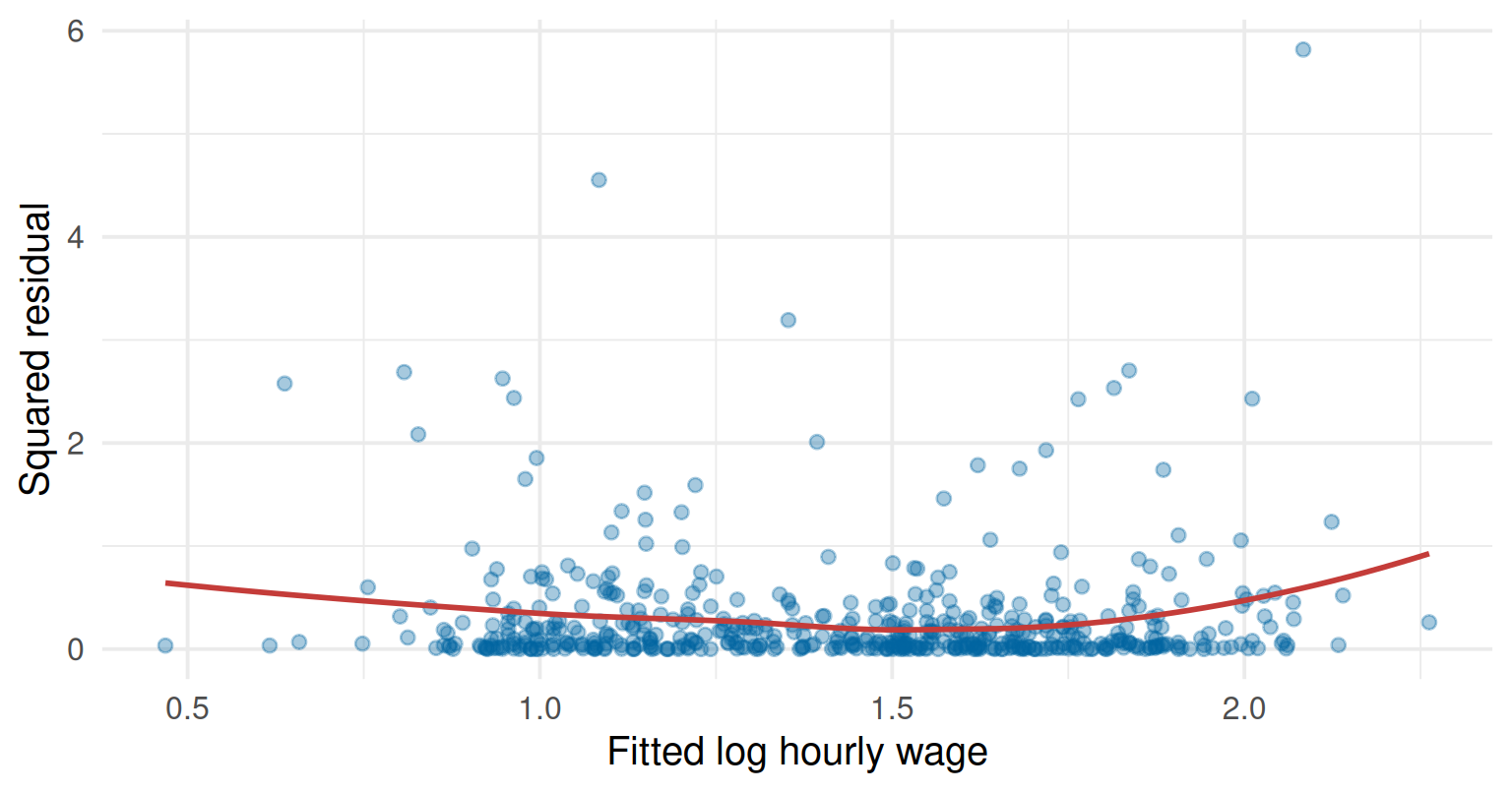

There is no clean monotonic fan shape. The smooth is mildly curved and several large squared residuals occur across the fitted-value range. This plot therefore does not supply decisive evidence either way. A residual plot is a diagnostic, not proof of homoskedasticity, and Lecture 3’s practical recommendation is still to use HC standard errors by default for a cross-section.

In this sample, HC1 makes the standard errors for educ and exper larger, the one for union smaller, and the one for male almost unchanged. Robust standard errors are not necessarily larger; they are designed to be valid under weaker variance assumptions, not automatically conservative.

HC1 does not change a biased coefficient, so it cannot repair omitted-variable bias. It also treats off-diagonal covariances as zero, so it does not allow errors to be correlated among workers at the same firm. That dependence calls for standard errors clustered by firm, provided the research design and number of clusters support that choice.

Which controls belong?

1. ability is a confounder: \(ability\rightarrow education\) and \(ability\rightarrow wage\). It should be controlled for, assuming it is measured well and precedes education.

2. In the stipulated data-generating process, experience affects wages but is independent of and not caused by education. It is a valid but irrelevant control for education bias. Omitting it does not bias the education coefficient. Including it may improve precision if it explains residual wage variation, but it can also consume degrees of freedom.

3. occupation is a mediator: \(education\rightarrow occupation\rightarrow wage\). Controlling for it blocks part of the total effect of education and changes the target toward a direct effect.

4. hired is a collider because education and raw talent both affect hiring. Conditioning on being hired opens a spurious association between education and talent. Restricting the sample to hired workers is already conditioning on this collider.

5. Adding experience should leave the education estimate near 1.85 because experience is unrelated to education in this example. Adding ability should remove the upward omitted-variable bias and move the coefficient down toward the true value of 1.2.

6. Including ability improves credibility by addressing confounding. But if ability and education are strongly correlated, the auxiliary \(R_j^2\) is high, \(1-R_j^2\) is small, and the variance and standard error of the education estimate rise. The needed control can therefore reduce bias while reducing precision.

Interpreting an interaction

1. For non-homeowners, homeowner is zero:

\[ \widehat{donations}=50+5\,age. \]

One additional year of age is associated with €5 more in predicted donations.

2. For homeowners, homeowner is one:

\[ \widehat{donations} =(50+150)+(5+3)age =200+8\,age. \]

One additional year of age is associated with €8 more in predicted donations.

3. The interaction coefficient is the difference between the age slopes. The predicted age–donations slope is €3 larger for homeowners.

4. At any age, the homeowner–non-homeowner difference is

\[ 150+3\,age. \]

At age 50 this is \(150+3(50)=€300\).

5. Equal slopes requires the single restriction \(H_0:\beta_{homeowner\times age}=0\), so use a \(t\)-test. For the two lines to be identical at every age, both the intercept difference and slope difference must vanish:

\[ H_0:\beta_{homeowner}=\beta_{homeowner\times age}=0. \]

That is a joint \(F\)- or Wald test.

Choosing standard errors

1. Use HC1 standard errors. The changing variance of electricity use is heteroskedasticity in a cross-section.

2. Use cluster-robust standard errors at the country level. Both the errors and GDP are likely correlated over time within a country; the independent units for this dependence structure are countries, not country-years.

3. Use cluster-robust standard errors at the school level. Treatment is assigned by school, so \(\rho_x=1\), and shared teachers and resources imply within-school error correlation.

4. Clustering by school remains a safe way to allow the known within-school dependence, but assigning treatment independently within schools makes \(\rho_x\) close to zero. The shared school shock then largely cancels when comparing treated and untreated students within the same school. Classical or HC standard errors need not be severely too small in this idealized design, and clustering may change little.

5. For study 3,

\[ \frac{se_C}{se_{OLS}} \approx\sqrt{1+0.20(1)(25-1)} =\sqrt{5.8} \approx 2.41. \]

The classical standard error is therefore predicted to be about 2.4 times too small.

6. HC1 allows each diagonal variance to differ but still sets covariances between different students to zero. It misses the within-school cross-products created by a shared shock. With school-level treatment, adding more students to a school supplies much less new treatment information than adding more schools, so precision is governed primarily by the number of independent schools.

Self-study

Categories and the dummy-variable trap

1. At five years of experience, predicted salaries are:

Education	Prediction
High School	\(32{,}000+1{,}000(5)=€37{,}000\)
Bachelors	\(32{,}000+12{,}000+1{,}000(5)=€49{,}000\)
Masters	\(32{,}000+24{,}000+1{,}000(5)=€61{,}000\)
PhD	\(32{,}000+38{,}000+1{,}000(5)=€75{,}000\)

2. Holding experience constant, a worker with a master’s degree has a predicted salary €24,000 higher than a worker with a high-school education. It is a difference from the baseline, not the master’s worker’s predicted salary.

3. For every observation,

\[ HighSchool+Bachelors+Masters+PhD=1. \]

The right-hand side duplicates the intercept exactly. Including all four dummies and an intercept therefore creates perfect multicollinearity, so the separate coefficients are not identified.

4. With Bachelors as the baseline, the same fitted model is

\[ \widehat{salary} =44{,}000-12{,}000HighSchool+12{,}000Masters +26{,}000PhD+1{,}000exper. \]

5. The coefficient labels and their individual baseline comparisons change. The predicted values, residuals, \(R^2\), and joint significance of education do not. With High School as baseline the joint null is

\[ H_0:\beta_{Bachelors}=\beta_{Masters}=\beta_{PhD}=0. \]

With Bachelors as baseline, the equivalent null sets the High School, Masters, and PhD coefficients jointly to zero. Both test whether all education categories have the same conditional mean.

A joint hypothesis test

1. The unrestricted model is

\[ wage_i=\beta_0+\beta_1educ_i+\beta_2exper_i +\beta_3exper\_sq_i+u_i. \]

The restricted model imposes \(\beta_2=\beta_3=0\):

\[ wage_i=\beta_0+\beta_1educ_i+u_i. \]

There are \(q=2\) restrictions.

2. The unrestricted model estimates \(p=4\) parameters, so its residual degrees of freedom are \(100-4=96\):

\[ F =\frac{(880-800)/2}{800/96} =\frac{40}{8.333} =4.8. \]

3. The \(p\)-value is about 0.010, below 0.05. We reject the joint null: exper and exper_sq matter jointly, conditional on education.

4. The \(F\)-test evaluates the two coefficients together and accounts for the covariance between their estimates. With highly correlated regressors, neither coefficient may be precisely separated from the other, even though dropping both makes model fit substantially worse. Two individual \(t\)-tests do not answer the joint question.

5. No. The SSR-based statistic uses the classical homoskedastic variance assumptions. With heteroskedasticity, request an HC-robust Wald test of the same two restrictions from the robust model.

Takeaways

What should you be able to do now?

1. Interpret a coefficient in a multiple regression as a ceteris paribus comparison, and defend each control by its causal role rather than by its contribution to \(R^2\).
2. Estimate the same specification with classical, HC1, and cluster-robust standard errors in R or Python, and say exactly which reported quantities change.
3. Test one restriction with a \(t\)-test and several jointly with an \(F\)-test, and explain why the two can point in different directions.
4. Read, predict from, and rewrite models containing categorical regressors and interactions, including a change of baseline category.
5. Choose a level of clustering from the design of a study, and use the Moulton factor to anticipate how far classical inference would be off.