Solutions Tutorial 6: Difference-in-Differences (Entrepreneurship Track)

Retrieval practice

  1. \(Y_i(1)\) is the outcome with treatment and \(Y_i(0)\) the outcome without treatment; an individual receives only one treatment status, so the other potential outcome is unobserved.
  2. The difference equals the ATT, \(E[Y(1)-Y(0)\mid D=1]\), plus selection bias, \(E[Y(0)\mid D=1]-E[Y(0)\mid D=0]\).
  3. DiD is \((\bar Y_{1,post}-\bar Y_{1,pre})-(\bar Y_{0,post}-\bar Y_{0,pre})\); the control group’s change estimates the treated group’s counterfactual change without treatment.
  4. \(\beta_0\) is the control group’s pre-treatment mean, \(\beta_1\) the initial treated-control difference, \(\beta_2\) the control group’s change and \(\beta_3\) the DiD contrast.
  5. Parallel trends requires equal average changes in untreated potential outcomes across groups; pre-treatment diagnostics cannot observe the treated group’s post-treatment outcome without treatment.

Solutions

1. Potential outcomes for irrigation

Part 1: The potential outcomes

\(Y_i(1)\) is farm \(i\)’s yield if it uses the new irrigation system. \(Y_i(0)\) is the same farm’s yield if it continues without that system. Both refer to the same period and farm under different treatment states.

Part 2: The individual effect

\[\tau_i=Y_i(1)-Y_i(0).\]

This is the effect of the new system on yield for farm \(i\).

Part 3: The unobserved counterfactual

If a farm adopts the system, we observe \(Y_i(1)\) and cannot observe its yield in the same period without adoption, \(Y_i(0)\). For a non-adopting farm the reverse applies. We therefore cannot calculate \(\tau_i\) directly from observed outcomes. An empirical design uses comparisons across farms or periods to identify an average effect under stated assumptions.

2. Selection bias in a job training comparison

Part 1: Decomposing the difference in means

Let \(\Delta_{obs}\) denote the observed difference in mean earnings between participants and non-participants. Observed outcomes satisfy

\[ \Delta_{obs}=E[Y(1)\mid D=1]-E[Y(0)\mid D=0]. \]

Adding and subtracting the same counterfactual mean leaves the expression unchanged:

\[ \begin{aligned} \Delta_{obs} &= \underbrace{E[Y(1)\mid D=1]-E[Y(0)\mid D=1]}_{\text{ATT}} +\underbrace{E[Y(0)\mid D=1]-E[Y(0)\mid D=0]}_{\text{selection bias}}\\ &= \text{ATT}+\text{selection bias}. \end{aligned} \]

The first two terms form the ATT, comparing participants’ earnings with and without training. The last two terms form selection bias, comparing the two groups’ earnings without training.

Part 2: Interpreting positive selection bias

Positive selection bias means that participants would have earned more than non-participants even without training. For example, participants may have greater prior skills that raise earnings independently of the programme. A comparison after training then overstates the ATT by attributing this pre-existing advantage to training.

3. House prices after a subway opening

Part 1: Calculating DiD

Prices rise by \(520-450=70\) in the treated neighbourhood and by \(460-420=40\) in the control neighbourhood. Therefore,

\[\hat\tau_{DiD}=70-40=30.\]

Part 2: The trend and counterfactual

The estimated secular trend is the control group’s increase of 40, or $40,000. Under parallel trends, the treated neighbourhood’s counterfactual price after opening is \(450+40=490\), or $490,000.

Part 3: Interpreting the estimate

The treated neighbourhood’s observed price exceeds that counterfactual by \(520-490=30\), or $30,000. This estimates the ATT if untreated prices would have changed equally across neighbourhoods, there was no anticipation or spillover, and the houses compared remained comparable over time. Without these assumptions, 30 is a descriptive difference in changes.

4. Reading the environmental-policy coefficients

Part 1: The control group’s initial mean

Setting Treat = 0 and Post = 0 leaves the intercept: 75.2 index points.

Part 2: The initial group difference

Before adoption, the treated provinces’ mean index is 5.5 points higher than the control provinces’ mean. Their initial mean is \(75.2+5.5=80.7\).

A baseline difference alone does not establish whether assignment was random. Random assignment can produce differences by chance in a finite sample; the assignment process and its statistical implications must be assessed separately. DiD allows an initial level difference under parallel trends.

Part 3: The control group’s change

The coefficient \(-8.1\) is the control group’s change from before to after adoption. Its post-treatment mean is \(75.2-8.1=67.1\). Under parallel trends, this change estimates the treated group’s change without the policy.

Part 4: The policy contrast

The interaction coefficient is \(-4.3\) index points. The treated group’s change is \(-8.1-4.3=-12.4\); subtracting the control group’s change gives \(-12.4-(-8.1)=-4.3\).

Under the identifying assumptions, the policy reduced the index by 4.3 points relative to the no-policy counterfactual. Whether that represents better air quality depends on the index definition. No standard error or confidence interval is supplied, so statistical significance cannot be assessed.

6. Union membership and wages

Part 1: Defining a balanced two-period sample

Keep women with observed wages and union status in both years and non-union status in 77. Treat is their union status in 78 and is constant within a woman; Post equals one for year 78. This gives 74 treated women and 801 control women, each observed twice: 875 women and 1,750 observations.

Code
library(haven)
library(dplyr)
library(fixest)

nlswork <- read_dta(
  "https://empirical-economics.netlify.app/tutorials/datafiles/nlswork.dta"
)
sample <- nlswork |>
  filter(year %in% c(77, 78), !is.na(union), !is.na(ln_wage)) |>
  group_by(idcode) |>
  filter(n() == 2, n_distinct(year) == 2) |>
  filter(union[year == 77] == 0) |>
  mutate(Treat = as.integer(union[year == 78]),
         Post = as.integer(year == 78)) |>
  ungroup()

sample |> distinct(idcode, Treat) |> count(Treat)
Code
import numpy as np
import pandas as pd
import statsmodels.formula.api as smf

nlswork = pd.read_stata(
    "https://empirical-economics.netlify.app/tutorials/datafiles/nlswork.dta"
)
nlswork["ln_wage"] = nlswork["ln_wage"].astype(float)
sample = nlswork.loc[nlswork["year"].isin([77, 78])].dropna(
    subset=["union", "ln_wage"]
)
status = sample.pivot(index="idcode", columns="year", values="union").dropna()
status = status.loc[status[77] == 0]
sample = sample.loc[sample["idcode"].isin(status.index)].copy()
sample["Treat"] = sample["idcode"].map(status[78]).astype(int)
sample["Post"] = (sample["year"] == 78).astype(int)

print(sample.drop_duplicates("idcode").groupby("Treat").size())

Part 2: The four means

Group Mean log wage, 77 Mean log wage, 78 Change
Control 1.668938 1.729596 0.060658
Treated 1.679984 1.777452 0.097468

Thus \(\hat\tau_{DiD}=0.097468-0.060658=\mathbf{0.036810}\) log points.

Code
means <- sample |>
  group_by(Treat, Post) |>
  summarise(mean_log_wage = mean(ln_wage), .groups = "drop")
changes <- means |>
  group_by(Treat) |>
  summarise(change = mean_log_wage[Post == 1] -
                     mean_log_wage[Post == 0], .groups = "drop")
tau <- with(changes, change[Treat == 1] - change[Treat == 0])
print(means)
print(tau)
Code
means = sample.groupby(["Treat", "Post"])["ln_wage"].mean().unstack("Post")
changes = means[1] - means[0]
tau = changes.loc[1] - changes.loc[0]
print(means)
print(tau)

Part 3: The regression and interpretation

Term Estimate Person-clustered SE
Intercept 1.6689 0.0140
Treat 0.0110 0.0459
Post 0.0607 0.0094
Treat:Post 0.0368 0.0414

The interaction equals the manual estimate. Wages for the women who joined a union increased by about 3.7% more than wages for the controls, using \(100\hat\tau\) as a log-point approximation. Exponentiating gives \(100(e^{0.036810}-1)=3.75\%\), a contrast in geometric mean wage growth.

The clustered p-value is approximately 0.374 and the 95% confidence interval is approximately \([-0.044,0.118]\) log points. The estimate is compatible with both a decrease and an increase; non-rejection does not establish that the effect is zero.

A causal interpretation requires parallel untreated wage trends, no anticipation and no spillovers. Joining a union may coincide with changing jobs or other wage shocks. Two periods alone provide no pre-trend check, and clustering changes estimated uncertainty without addressing selection into membership.

Code
did_model <- feols(ln_wage ~ Treat * Post, data = sample, vcov = ~idcode)
etable(did_model)
confint(did_model, parm = "Treat:Post")
stopifnot(isTRUE(all.equal(unname(coef(did_model)["Treat:Post"]), tau)))
Code
did_model = smf.ols("ln_wage ~ Treat * Post", data=sample).fit(
    cov_type="cluster", cov_kwds={"groups": sample["idcode"]}, use_t=True
)
print(pd.DataFrame({
    "Estimate": did_model.params,
    "Clustered SE": did_model.bse,
    "p-value": did_model.pvalues,
}))
print(did_model.conf_int().loc["Treat:Post"])
assert np.isclose(did_model.params["Treat:Post"], tau)

7. Cohort differences before treatment

Part 1: Importing the supplied categories

Exclude Post and observations with missing outcomes or group indicators. The usable pre-treatment sample has 20,861 observations. Convert the labelled Stata variable explicitly in R so that labels such as -1 are used in place of their underlying numeric codes.

Code
library(haven)
library(dplyr)
library(ggplot2)

did_data <- read_dta(
  "https://empirical-economics.netlify.app/tutorials/datafiles/duflo_did_data.dta"
)
pre <- did_data |>
  mutate(cohort = as.character(as_factor(cohort))) |>
  filter(cohort %in% c("-4", "-3", "-2", "-1"),
         !is.na(yeduc), !is.na(treated)) |>
  mutate(cohort = factor(cohort, levels = c("-4", "-3", "-2", "-1")))
nrow(pre)
Code
import pandas as pd
import matplotlib.pyplot as plt
import statsmodels.formula.api as smf

did_data = pd.read_stata(
    "https://empirical-economics.netlify.app/tutorials/datafiles/duflo_did_data.dta"
)
pre = did_data.loc[did_data["cohort"].isin(["-4", "-3", "-2", "-1"])].dropna(
    subset=["yeduc", "treated"]
).copy()
pre["cohort"] = pre["cohort"].cat.remove_unused_categories()
print(len(pre))

Part 2: The pre-treatment plot

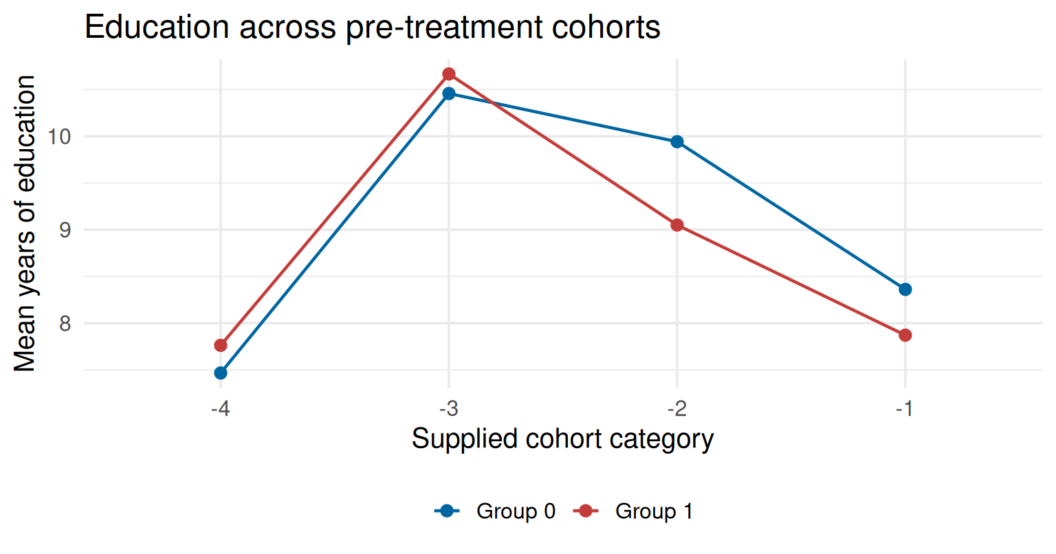
Mean years of education for groups 0 and 1 across four cohort categories. The group gap changes sign between cohorts -3 and -2.

The group difference is not stable. Group 1 has about 0.30 more years of education in cohort -4 and 0.21 more in -3, but 0.89 fewer in -2 and 0.49 fewer in -1. The gap changes sign, providing evidence against equal pre-treatment changes for these groups. The -3 category is also small, with only 106 observations across both groups.

Code
means_pre <- pre |>
  group_by(cohort, treated) |>
  summarise(mean_yeduc = mean(yeduc), .groups = "drop")
ggplot(means_pre, aes(cohort, mean_yeduc, group = factor(treated),
                      colour = factor(treated))) +
  geom_line(linewidth = 0.8) + geom_point(size = 2.5) +
  scale_colour_manual(values = c("0" = "#0066a1", "1" = "#c43c39"),
                      labels = c("Group 0", "Group 1")) +
  labs(title = "Education across pre-treatment cohorts",
       x = "Supplied cohort category", y = "Mean years of education", colour = NULL) +
  theme_minimal(base_size = 15) + theme(legend.position = "bottom")
Code
means_pre = pre.groupby(["cohort", "treated"], observed=True)["yeduc"].mean()
means_pre = means_pre.unstack("treated")
plt.rcParams.update({"font.size": 15})
fig, ax = plt.subplots(figsize=(8, 4.2), layout="constrained")
for group, colour in [(0, "#0066a1"), (1, "#c43c39")]:
    ax.plot(range(4), means_pre[group], marker="o", color=colour,
            label=f"Group {group}")
ax.set(xticks=range(4), xticklabels=["-4", "-3", "-2", "-1"],
       title="Education across pre-treatment cohorts",
       xlabel="Supplied cohort category", ylabel="Mean years of education")
ax.spines[["top", "right"]].set_visible(False)
ax.legend(frameon=False)
plt.show()
Part 3: The regression and joint null

For individual \(i\) in cohort \(c\), let \(D_i\) be the supplied group indicator and \(C_{ik}\) indicate membership in cohort \(k\). Using only the four pre-treatment categories, estimate

\[ Y_{ic}=\alpha+\eta D_i+\sum_{k=-4}^{-2}\gamma_k C_{ik}+\sum_{k=-4}^{-2}\delta_k(D_i C_{ik})+u_{ic}. \]

Cohort -1 is omitted from both sets of indicators, so \(\delta_{-1}=0\). The group difference in that category is \(\eta\). Each \(\delta_k\) measures how the group difference in cohort \(k\) differs from the reference gap.

The joint null is \(H_0:\delta_{-4}=\delta_{-3}=\delta_{-2}=0\). Under this null, the pre-treatment group gap is constant across the supplied categories.

Part 4: Estimating and interpreting the diagnostic

Interaction relative to cohort -1 Estimate Conventional SE
Group 1 × cohort -4 0.7857 0.1178
Group 1 × cohort -3 0.6996 0.7576
Group 1 × cohort -2 -0.4014 0.1573

The joint test gives \(F(3,20853)=28.268\), with \(p=3.11\times10^{-18}\). Reject a constant pre-treatment gap. These results raise concerns about using this comparison for DiD. They cannot directly test the unobserved post-treatment trend without treatment.

The conventional test here assumes independent, homoskedastic errors. A regional-policy study must account for shared shocks and treatment assignment within regions, usually by clustering at the appropriate regional level. Its standard errors and joint test could differ from this classroom diagnostic. The result above concerns the groups coded in this teaching extract and is not a conclusion about the published school-construction study.

Code
pre$cohort <- relevel(pre$cohort, ref = "-1")
pre_model <- lm(yeduc ~ cohort * treated, data = pre)
restricted <- lm(yeduc ~ cohort + treated, data = pre)
terms <- grep(":treated$", names(coef(pre_model)), value = TRUE)
print(coef(summary(pre_model))[terms, , drop = FALSE])
anova(restricted, pre_model)
Code
pre_model = smf.ols(
    "yeduc ~ C(cohort, Treatment(reference='-1')) * treated", data=pre
).fit()
terms = [name for name in pre_model.params.index if ":treated" in name]
print(pd.DataFrame({
    "Estimate": pre_model.params[terms],
    "Conventional SE": pre_model.bse[terms],
}))
joint_test = pre_model.f_test([f"{name} = 0" for name in terms])
print(joint_test)

Self-study

8. Threats to a scholarship comparison

Part 1: Anticipation

Students in City A may postpone enrollment until scholarships become available. Enrollment falls before introduction and rises when the programme starts. This violates the no-anticipation assumption if the nominal pre-treatment period is already affected by the announcement, contaminating the baseline comparison.

Part 2: Spillovers

Students from City B may move to City A to become eligible, changing enrollment rates in both cities. City B’s observed outcome is then affected by the scholarship programme and no longer represents an untreated comparison. The direction of bias depends on how migration changes the measured outcomes and denominators.

Part 3: Ashenfelter’s dip

Suppose a temporary local income shock reduces enrollment in City A, and the city introduces scholarships in response. Even without scholarships, enrollment would recover as the shock subsides. DiD attributes this untreated recovery to the programme if City B does not have the same recovery. The estimated scholarship effect is then biased upward.

The relevant dip is in the outcome being analysed, enrollment. A fall in family income creates this problem only if it produces a temporary enrollment decline followed by recovery.

9. The direction of fertilizer bias

Part 1: Assessing the pre-treatment pattern

Declining yields for adopters and stable yields for controls provide evidence against equal untreated changes before adoption. This weakens the credibility of parallel trends. It does not directly establish the post-treatment assumption, which concerns what adopters’ yields would have been without fertilizer.

Part 2: Deriving the bias

With no anticipation and no spillovers, add and subtract the treated farms’ missing post-treatment mean without adoption:

\[ \begin{aligned} \tau_{DiD} &= E[Y_{post}-Y_{pre}\mid D=1]-E[Y_{post}-Y_{pre}\mid D=0]\\ &= \text{ATT}+B, \end{aligned} \]

where

\[ \begin{aligned} \text{ATT} &= E[Y_{post}(1)-Y_{post}(0)\mid D=1],\\ B &= E[Y_{post}(0)-Y_{pre}(0)\mid D=1]-E[Y_{post}(0)-Y_{pre}(0)\mid D=0]. \end{aligned} \]

Under the stated continuation assumption, the first untreated change is negative and the second is zero. Thus \(B<0\) and \(\tau_{DiD}<\text{ATT}\): the positive DiD estimate underestimates the treatment effect.

DiD uses the control group’s flat trend to estimate the treated group’s counterfactual. If untreated yields would actually have declined, that counterfactual is too high, making the estimated improvement too small. This sign requires the assumed continuation of the declining trend; the pre-treatment graph alone does not determine the bias after adoption.

Takeaways

What should you be able to do now?

  1. Define potential outcomes and decompose a difference in means into the ATT and selection bias.
  2. Calculate DiD from four means and interpret all four regression coefficients.
  3. State the parallel trends assumption and explain the limits of pre-treatment diagnostics.
  4. Construct a two-period sample, estimate DiD in R or Python and report uncertainty using an appropriate clustering level.
  5. Estimate and jointly test pre-treatment interactions relative to an omitted reference category.
  6. Explain anticipation, spillovers and outcome-dependent treatment timing, and derive the direction of bias under a stated untreated trend.