# Load the packages
library(haven)
library(dplyr)

# 1. Load the data from the URL
url <- "https://empirical-economics.netlify.app/tutorials/datafiles/nlswork.dta"
nlswork <- read_dta(url)

# 2. Filter for years 77 and 78
nlswork <- nlswork |>
  filter(year == 77 | year == 78)

# 3. Create the 'post' dummy variable
nlswork <- nlswork |>
  mutate(post = as.integer(year == 78))

# 4. Identify the treated and control group IDs
ids_union0_post0 <- nlswork |>
  filter(union == 0, post == 0) |>
  distinct(idcode) |>
  pull(idcode)

ids_union1_post1 <- nlswork |>
  filter(union == 1, post == 1) |>
  distinct(idcode) |>
  pull(idcode)

ids_union0_post1 <- nlswork |>
  filter(union == 0, post == 1) |>
  distinct(idcode) |>
  pull(idcode)

treated_ids <- intersect(ids_union0_post0, ids_union1_post1)
control_ids <- intersect(ids_union0_post0, ids_union0_post1)

# 5. Create 'treated' and 'control' dummy variables
nlswork <- nlswork |>
  mutate(
    treated = as.integer(idcode %in% treated_ids),
    control = as.integer(idcode %in% control_ids)
  )

# 6. Keep only observations that are in either the treated or control group
nlswork <- nlswork |>
filter(treated + control == 1)Solutions Tutorial 6: Difference-in-Differences (Finance and Entrepreneurship Tracks)
Retrieval practice
- \(Y_i(1)\) is the outcome if \(i\) is treated and \(Y_i(0)\) the outcome if \(i\) is not; whichever one is not realised for that individual is the counterfactual.
- Into the ATT, \(E[Y_i(1)-Y_i(0)\mid T_i=1]\), plus selection bias, \(E[Y_i(0)\mid T_i=1]-E[Y_i(0)\mid T_i=0]\).
- \(\tau_{DiD}=(\hat Y_{T,Post}-\hat Y_{T,Pre})-(\hat Y_{C,Post}-\hat Y_{C,Pre})\); the control group’s change stands in for the trend the treated group would have followed without the treatment.
- \(\beta_3\), the coefficient on the interaction \(D_i\times Post_t\).
- That the average untreated outcome of the treated and control groups would have moved in parallel; it involves the unobserved post-treatment counterfactual for the treated, so it can only be supported by pre-treatment evidence, never verified.
Solutions
The Effect of Union Membership on Wages
- For this exercise, define the “treatment group” as women who were non-union in
year77 but became union members byyear78. The “control group” will be women who were non-union in bothyear77 andyear78. Create the relevant dummy variables (TreatandPost) for this 2x2 setup (Pre = 77, Post = 78).
import pandas as pd
import numpy as np
# Load the data for the year 77 and 78
url = "https://empirical-economics.netlify.app/tutorials/datafiles/nlswork.dta"
nlswork = pd.read_stata(url).query("year == 77 or year == 78")

#create the post dummy
nlswork['post'] = (nlswork['year'] == 78).astype(int)

# Create separate dummies for treated and control
ids_union0_post0 = nlswork.loc[(nlswork['union'] == 0) & (nlswork['post'] == 0), 'idcode'].unique()
ids_union1_post1 = nlswork.loc[(nlswork['union'] == 1) & (nlswork['post'] == 1), 'idcode'].unique()
ids_union0_post1 = nlswork.loc[(nlswork['union'] == 0) & (nlswork['post'] == 1), 'idcode'].unique()

treated_ids = np.intersect1d(ids_union0_post0, ids_union1_post1)
control_ids = np.intersect1d(ids_union0_post0, ids_union0_post1)

nlswork['treated'] = nlswork['idcode'].isin(treated_ids).astype(int)
nlswork['control'] = nlswork['idcode'].isin(control_ids).astype(int)

#Keep only observations that meet either the conditions for treated or control
nlswork = nlswork[(nlswork.treated+nlswork.control) == 1]- Manually calculate the four means for the 2x2 DiD table (\(\hat{Y}_{T, Pre}\), \(\hat{Y}_{T, Post}\), \(\hat{Y}_{C, Pre}\), \(\hat{Y}_{C, Post}\)) and compute the DiD estimate.
summary_tab <- nlswork |>
    group_by(treated, post) |>
    summarize(mean_ln_wage = mean(ln_wage, na.rm = TRUE))
`summarise()` has regrouped the output.
ℹ Summaries were computed grouped by treated and post.
ℹ Output is grouped by treated.
ℹ Use `summarise(.groups = "drop_last")` to silence this message.
ℹ Use `summarise(.by = c(treated, post))` for per-operation grouping
(`?dplyr::dplyr_by`) instead.print(summary_tab)# A tibble: 4 × 3
# Groups: treated [2]
treated post mean_ln_wage
<int> <int> <dbl>
1 0 0 1.67
2 0 1 1.73
3 1 0 1.68
4 1 1 1.78tau_did <- (
summary_tab$mean_ln_wage[summary_tab$treated == 1 & summary_tab$post == 1] -
summary_tab$mean_ln_wage[summary_tab$treated == 1 & summary_tab$post == 0] -
(summary_tab$mean_ln_wage[summary_tab$treated == 0 & summary_tab$post == 1] -
summary_tab$mean_ln_wage[summary_tab$treated == 0 & summary_tab$post == 0])
)
print(tau_did)[1] 0.03681027# Calculate group means, reset index, and sort to ensure correct order
did_table = nlswork.groupby(['treated', 'post'])['ln_wage'].mean().reset_index()
did_table = did_table.sort_values(['treated', 'post'])
# Assign descriptive labels
did_table.index = ['Control_Pre', 'Control_Post', 'Treated_Pre', 'Treated_Post']
print(did_table) treated post ln_wage
Control_Pre 0 0 1.668938
Control_Post 0 1 1.729596
Treated_Pre 1 0 1.679984
Treated_Post 1 1 1.777452
tau_did = (
    nlswork.loc[(nlswork['treated'] == 1) & (nlswork['post'] == 1), 'ln_wage'].mean() -
    nlswork.loc[(nlswork['treated'] == 1) & (nlswork['post'] == 0), 'ln_wage'].mean() -
    (nlswork.loc[(nlswork['treated'] == 0) & (nlswork['post'] == 1), 'ln_wage'].mean() -
    nlswork.loc[(nlswork['treated'] == 0) & (nlswork['post'] == 0), 'ln_wage'].mean())
)

print(tau_did)0.03680992- Estimate the DiD effect by running the regression \(Y_{it} = \beta_0 + \beta_1 Treat_i + \beta_2 Post_t + \beta_3(Treat_i \times Post_t) + \epsilon_{it}\). Confirm that the coefficient \(\hat{\beta}_3\) matches your manual calculation. Report and interpret the result.
library(fixest)
did_model <- feols(ln_wage ~ treated + post + treated:post, data = nlswork)
etable(did_model)
did_model
Dependent Var.: ln_wage
Constant 1.669*** (0.0136)
treated 0.0111 (0.0467)
post 0.0607** (0.0192)
treated x post 0.0368 (0.0660)
_______________ _________________
S.E. type IID
Observations 1,750
R2 0.00748
Adj. R2 0.00577
---
Signif. codes: 0 '***' 0.001 '**' 0.01 '*' 0.05 '.' 0.1 ' ' 1import pyfixest as pf
# tau_did can be estimated as the interaction of treated and post
# with treated*post pyfixest includes the main effects (treated and post)
# as well as the interaction term denoted as treated:post in the output
did_model = pf.feols("ln_wage ~ treated*post", data=nlswork)
did_model.summary()###
Estimation: OLS
Dep. var.: ln_wage, Fixed effects: 0
Inference: iid
Observations: 1750
| Coefficient | Estimate | Std. Error | t value | Pr(>|t|) | 2.5% | 97.5% |
|:--------------|-----------:|-------------:|----------:|-----------:|-------:|--------:|
| Intercept | 1.669 | 0.014 | 122.918 | 0.000 | 1.642 | 1.696 |
| treated | 0.011 | 0.047 | 0.237 | 0.813 | -0.081 | 0.103 |
| post | 0.061 | 0.019 | 3.159 | 0.002 | 0.023 | 0.098 |
| treated:post | 0.037 | 0.066 | 0.557 | 0.577 | -0.093 | 0.166 |
---
RMSE: 0.384 R2: 0.007 The model shows that the estimated effect of union membership on wages for women who joined a union between 1977 and 1978 is equal to the manually calculated DiD estimate. This indicates that joining a union is associated with an increase in 0.0368 in log wages. However, the estimate is not statistically significant, suggesting that union membership has no significant effect on wages.
Event Study and Parallel Trends
Import the data into your statistical software of choice.
Plot the average educational attainment (
yeduc) for the high-construction and low-construction regions for the pre-treatment cohorts (-4 until -1). Does this visual evidence support the parallel trends assumption for a simple DiD analysis around 1989? Discuss what you see in the cohorts leading up to the treatment.
# 1. Install and load necessary libraries
library(ggplot2)
library(dplyr)
library(haven)

# 2. Define the URL and read the Stata data file
url <- "https://empirical-economics.netlify.app/tutorials/datafiles/duflo_did_data.dta"
did_data <- read_dta(url)

# 3. Create the plot
# We first filter out the 'Post' cohort and convert 'treated' to a factor
# for better plotting and legend generation.
plot_data <- did_data |>
  mutate(cohort = as.factor(cohort)) |>
  filter(cohort != "4") |>
  group_by(cohort, treated) |>
  summarise(
    mean_yeduc = mean(yeduc, na.rm = TRUE)
  ) |>
  ungroup() # Ungrouping is a good practice after summarising

# You can print plot_data to see the summarized table
# print(plot_data)

# 4. Now, plot the aggregated data
ggplot(plot_data, aes(x = cohort, y = mean_yeduc, group = factor(treated), color = factor(treated))) +
  geom_line(linewidth = 1) +
  geom_point(size = 3) +
  labs(
    title = "Average Educational Attainment by Cohort and Treatment Status",
    x = "Cohort",
    y = "Average Educational Attainment",
    color = "Treated" # Sets the legend title
  ) +
  theme_minimal()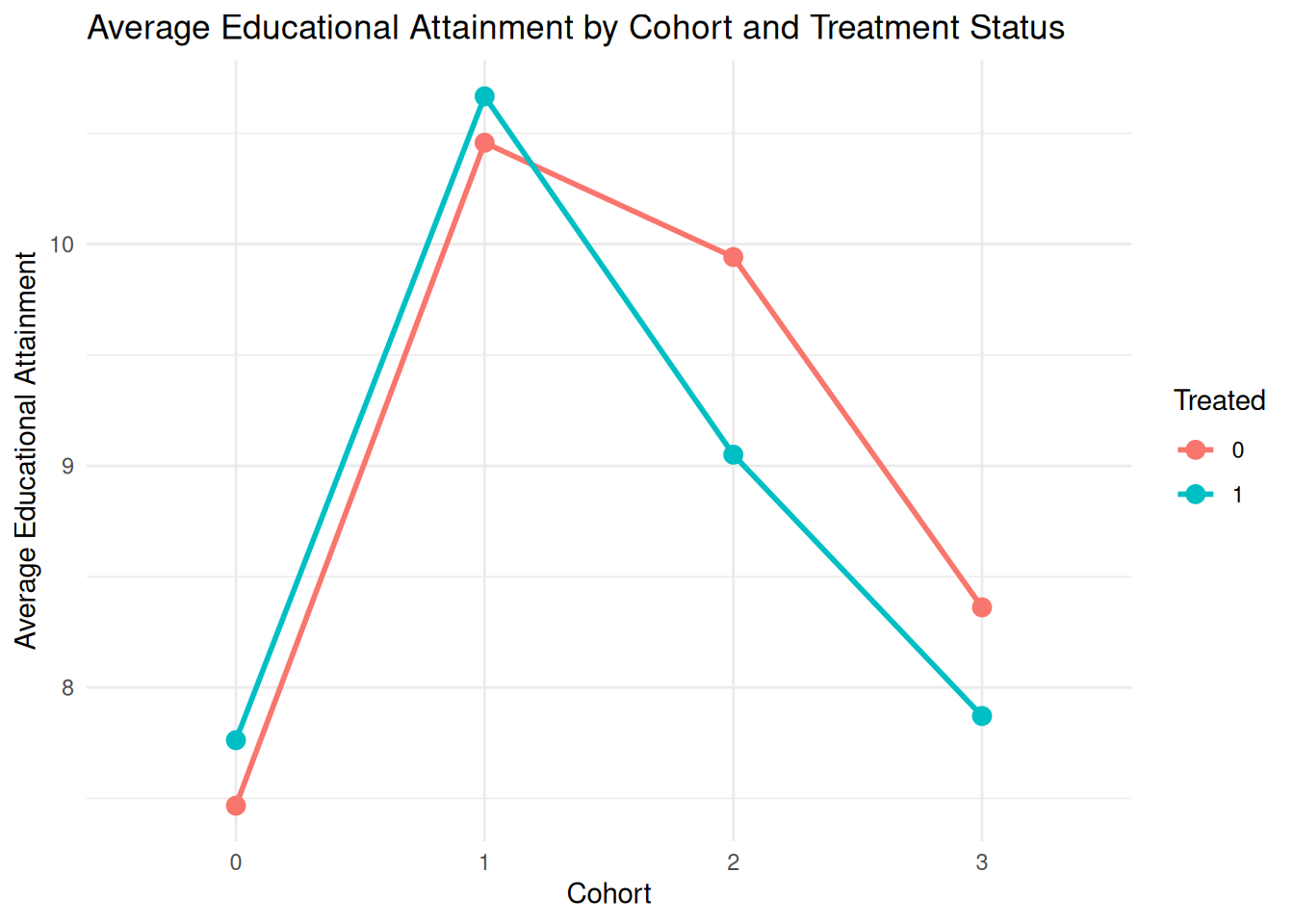
import pandas as pd
from matplotlib import pyplot as plt
import seaborn as sns

url = "https://empirical-economics.netlify.app/tutorials/datafiles/duflo_did_data.dta"
did_data = pd.read_stata(url)

# Plot the average educational attainment for high-construction and low-construction regions
plt.figure(figsize=(10, 6))
sns.lineplot(data=did_data.query("cohort != 'Post'"), x='cohort', y='yeduc', hue='treated', marker='o')
plt.title('Average Educational Attainment by Cohort and Treatment Status')
plt.xlabel('Cohort')
plt.ylabel('Average Educational Attainment')
plt.legend(title='Treated')
plt.show()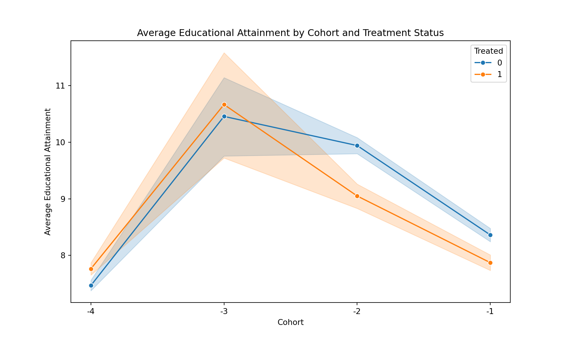
Even though visually, the trends for high-construction and low-construction regions appear to be similar in the pre-treatment cohorts (-4 to -1), there are some fluctuations that could raise concerns about the strict validity of the parallel trends assumption. For example, in cohort -2, there seems to be a noticeable divergence between the two groups. While the overall trend appears roughly parallel, these deviations suggest that a more formal statistical test is warranted to confirm the assumption.
- Briefly explain what parallel trends means in this context and outline how you would formally test for pre-trends using a regression framework. What coefficients would you be looking at, and what would you hope to find?
The parallel trends test asks: “Between cohorts of children who were all too old to be affected by the program, was the trend in educational attainment similar between high-construction and low-construction regions?” You would formally test for pre-trends by estimating a regression of the following form:\(Y_{ic} = \alpha + \sum_{c=-4}^{-1} \beta_c D_{c} \times Treated_i + \beta Treated_i + \sum_{c=-4}^{-1} \gamma_c D_c + u_{ic}\)
Where: \(c\) is the cohort, \(i\) is the individual, \(D_c\) is a dummy variable equal to 1 if the individual belongs to cohort \(c\), and \(Treated_i\) is a dummy variable equal to 1 if the individual comes from a high-construction region. You would be looking at the coefficients \(\beta_c\) for \(c = \{ -4, -3, -2, -1\}\). If the parallel trends assumption holds, you would hope to find that these coefficients are statistically indistinguishable from zero, indicating that there were no differential trends in educational attainment between high-construction and low-construction regions prior to the treatment period. You could also conduct an F-test to jointly test the null hypothesis that all \(\beta_c = 0\) for \(c = \{-4, -3, -2, -1\}\).
- Conduct this test. You must normalize \(\beta_{-1}=0\). Report and interpret your findings.
library(fixest)
# Analyze the pre-treatment data
pre_treatment_data <- did_data |>
    mutate(cohort = factor(cohort, labels = c("-4", "-3", "-2", "-1", "Post"))) |>
    filter(cohort != "Post")

parallel_trends <- feols(yeduc ~ i(cohort, treated, ref = "-1") + treated + i(cohort, ref="-1"), data = pre_treatment_data)

etable(parallel_trends)
parallel_trends
Dependent Var.: yeduc
Constant 8.361*** (0.0586)
treated x cohort = -4 0.7857*** (0.1178)
treated x cohort = -3 0.6996 (0.7576)
treated x cohort = -2 -0.4014* (0.1573)
treated -0.4900*** (0.0923)
cohort = -4 -0.8946*** (0.0751)
cohort = -3 2.096*** (0.4421)
cohort = -2 1.580*** (0.0927)
_____________________ ___________________
S.E. type IID
Observations 20,861
R2 0.04696
Adj. R2 0.04664
---
Signif. codes: 0 '***' 0.001 '**' 0.01 '*' 0.05 '.' 0.1 ' ' 1# Conduct an F-test for the joint significance of the interaction terms
joint_hypothesis <- c("cohort::-4:treated", "cohort::-3:treated", "cohort::-2:treated")
wald_result <- wald(parallel_trends, joint_hypothesis)Wald test, H0: joint nullity of cohort::-4:treated, cohort::-3:treated and cohort::-2:treated
stat = 28.3, p-value < 2.2e-16, on 3 and 20,853 DoF, VCOV: IID.# Print the result
print(wald_result$stat)[1] 28.26826print(wald_result$p)[1] 3.108391e-18import statsmodels.formula.api as smf
from statsmodels.iolib.summary2 import summary_col
# Filter the data
pre_treatment_data = did_data.query("cohort != 'Post'").copy()
# Focus only on post
pre_treatment_data['cohort'] = pre_treatment_data['cohort'].cat.remove_unused_categories()
# Now, run the model on this cleaned data. It will work as you expect.
parallel_trends_model = smf.ols(
"yeduc ~ C(cohort, Treatment(reference='-1')) * treated",
data=pre_treatment_data
).fit()
print(summary_col(parallel_trends_model,
stars=True,
model_names=["Parallel Trends Test"])
)
=======================================================================
                                                   Parallel Trends Test
-----------------------------------------------------------------------
Intercept                                          8.3615***
                                                   (0.0586)
C(cohort, Treatment(reference='-1'))[T.-4]         -0.8946***
                                                   (0.0751)
C(cohort, Treatment(reference='-1'))[T.-3]         2.0957***
                                                   (0.4421)
C(cohort, Treatment(reference='-1'))[T.-2]         1.5802***
                                                   (0.0927)
treated                                            -0.4900***
                                                   (0.0923)
C(cohort, Treatment(reference='-1'))[T.-4]:treated 0.7857***
                                                   (0.1178)
C(cohort, Treatment(reference='-1'))[T.-3]:treated 0.6996
                                                   (0.7576)
C(cohort, Treatment(reference='-1'))[T.-2]:treated -0.4014**
                                                   (0.1573)
R-squared                                          0.0470
R-squared Adj.                                     0.0466
=======================================================================
Standard errors in parentheses.
* p<.1, ** p<.05, ***p<.01
# Identify the interaction terms to test
# These are all the interaction terms, excluding the reference period.
interaction_terms = [c for c in parallel_trends_model.params.index if 'C(cohort' in c and 'treated' in c]
print("Testing the following interaction terms jointly:")Testing the following interaction terms jointly:print(interaction_terms)["C(cohort, Treatment(reference='-1'))[T.-4]:treated", "C(cohort, Treatment(reference='-1'))[T.-3]:treated", "C(cohort, Treatment(reference='-1'))[T.-2]:treated"]# Run the F-test
f_test_results = parallel_trends_model.f_test(interaction_terms)
print(f_test_results)<F test: F=28.268263009104043, p=3.1083908432155326e-18, df_denom=2.09e+04, df_num=3>The F-test decisively rejects the null hypothesis that all pre-treatment interaction terms are equal to zero (p-value < 0.01). This indicates that there are significant differences in the trends of educational attainment between high-construction and low-construction regions in the pre-treatment cohorts. Therefore, the parallel trends assumption does not hold in this context, suggesting that a simple DiD analysis may yield biased estimates of the treatment effect.
Decomposing the Naive Estimator
- Derivation of ATT and Selection Bias
The simple difference-in-means estimator, also known as the naive estimator, is a biased estimator for the Average Treatment Effect on the Treated (ATT). Here is the full derivation that decomposes this difference into the ATT and the Selection Bias term.
The derivation begins with the identity that the observed difference in mean outcomes between the treated and control groups is equivalent to the difference in their potential outcomes.
\(E[Y|T=1] - E[Y|T=0] = E[Y(1)|T=1] - E[Y(0)|T=0]\)
To isolate the ATT, we need to introduce the counterfactual outcome for the treated group, which is what their outcome would have been had they not received the treatment, represented as \(E[Y(0)|T=1]\). We do this by adding and subtracting this term from the right-hand side of the equation. This is a common algebraic trick that does not change the value of the expression.
\[ E[Y|T=1] - E[Y|T=0] = E[Y(1)|T=1] - E[Y(0)|T=0] + E[Y(0)|T=1] - E[Y(0)|T=1] \]
Next, we rearrange the terms to group the components that form the ATT and the selection bias.
\[ E[Y|T=1] - E[Y|T=0] = (E[Y(1)|T=1] - E[Y(0)|T=1]) + (E[Y(0)|T=1] - E[Y(0)|T=0]) \]
The rearranged expression now clearly shows the two components:
- Average Treatment Effect on the Treated (ATT): The first part of the expression, \((E[Y(1)|T=1] - E[Y(0)|T=1])\), is the definition of the ATT. It represents the difference in the potential outcome with treatment and the potential outcome without treatment for those who actually received the treatment.
- Selection Bias: The second part of the expression, \((E[Y(0)|T=1] - E[Y(0)|T=0])\), is the selection bias. It represents the difference in the potential outcome without treatment between the treated group and the control group. In other words, it captures the pre-existing differences between the two groups that would exist even in the absence of the treatment.
Therefore, the final decomposition is:
\(E[Y|T=1] - E[Y|T=0] = \text{ATT} + \text{Selection Bias}\)
In the context of a job training program, the selection bias term, \(E[Y(0)|T=1] - E[Y(0)|T=0]\), represents the difference in potential earnings (if neither group had received training) between those who chose to enroll in the program and those who did not.
- \(E[Y(0)|T=1]\) is the average earnings that the individuals who participated in the training program would have had if they had not participated.
- \(E[Y(0)|T=0]\) is the average earnings of the individuals who did not participate in the training program.
A positive selection bias in this context would imply that even without the training program, the group that chose to participate would have had higher earnings than the group that did not. This could be because the participants are, on average, more motivated, have a stronger work ethic, or possess other unobserved characteristics that are correlated with higher earnings. In this scenario, simply comparing the average earnings of the two groups after the program would overstate the true effect of the training because you would be incorrectly attributing the pre-existing earnings advantage of the treatment group to the program itself.
The 2x2 Calculation
- Difference-in-Differences Estimate Calculation
The Difference-in-Differences (DiD) estimate is calculated by comparing the change in the outcome for the treatment group to the change in the outcome for the control group over the same period.
Step 1: Calculate the change in house prices for the Treatment group.
\(\Delta_{\text{Treatment}} = \text{After}_{\text{Treatment}} - \text{Before}_{\text{Treatment}}\)
\(\Delta_{\text{Treatment}} = 520 - 450 = 70\)
Step 2: Calculate the change in house prices for the Control group.
\(\Delta_{\text{Control}} = \text{After}_{\text{Control}} - \text{Before}_{\text{Control}}\)
\(\Delta_{\text{Control}} = 460 - 420 = 40\)
Step 3: Calculate the Difference-in-Differences estimate.
\(\tau_{DiD} = \Delta_{\text{Treatment}} - \Delta_{\text{Control}}\)
\(\tau_{DiD} = 70 - 40 = 30\)
The Difference-in-Differences estimate for the effect of the subway line on house prices is $30,000.
- Secular Trend in House Prices
The “secular trend” in house prices refers to the change in prices that would have occurred even in the absence of the treatment (the new subway line). In a DiD analysis, this is estimated by the change in the outcome for the control group.
Secular Trend = \(\Delta_{\text{Control}} = 460 - 420 = 40\)
According to this data, the secular trend in house prices is an increase of $40,000.
3.. Conclusion on the Causal Effect
Based on the DiD estimate of $30,000, the conclusion is that the new subway line caused an increase in local house prices of $30,000 on average. This is because the house prices in the treatment neighborhood increased by $30,000 more than in the similar neighborhood that did not get the subway line.
Applying Potential Outcomes
In the context of the irrigation system study, the potential outcomes for a farm i are:
- \(Y_i(1)\): This represents the crop yield that farm i would have if it were to use the new irrigation system.
- \(Y_i(0)\): This represents the crop yield that farm i would have if it were to not use the new irrigation system (i.e., continue with its existing irrigation method).
The individual causal effect (\(\tau_i\)) for a single farm i is the difference between its two potential outcomes:
\(\tau_i = Y_i(1) - Y_i(0)\)
This represents the true, individual-level impact of the new irrigation system on the crop yield for that specific farm.
The “fundamental problem of causal inference” is that for any individual farm i, we can only ever observe one of its potential outcomes.
In the irrigation example, a farm either adopts the new irrigation system or it does not.
- If the farm adopts the new system, we observe \(Y_i(1)\), but we will never know what its yield would have been without it, \(Y_i(0)\).
- If the farm does not adopt the new system, we observe \(Y_i(0)\), but we will never know what its yield would have been with it, \(Y_i(1)\).
Because we cannot simultaneously observe both potential outcomes for the same farm at the same time, we can never directly calculate the individual causal effect, \(\tau_i\).
The Parallel Trends Assumption
The parallel trends assumption can be expressed mathematically using potential outcomes as:
\(E[Y(0)_{\text{post}} - Y(0)_{\text{pre}} | T=1] = E[Y(0)_{\text{post}} - Y(0)_{\text{pre}} | T=0]\)
Where:
- \(Y(0)\) is the potential outcome in the absence of treatment.
- ‘post’ and ‘pre’ denote the after and before periods, respectively.
- \(T=1\) indicates the treatment group and \(T=0\) indicates the control group.
In plain English, the parallel trends assumption means that in the absence of the treatment, the average outcome for the treatment group would have changed over time in the same way as the average outcome for the control group. It does not mean that the two groups must have the same level of the outcome, but that their trends would be parallel.
This assumption is essential for the DiD strategy because it allows us to use the change in the control group’s outcome as a proxy for the counterfactual change in the treatment group’s outcome. The unobservable counterfactual it allows us to estimate is what the trend in the outcome for the treatment group would have been if they had not received the treatment.
If data from several years before the treatment was implemented were available, you could visually build evidence for the credibility of the parallel trends assumption by plotting the average outcome for both the treatment and control groups over time. If the two lines move in a parallel fashion in the pre-treatment period, it provides visual support for the assumption that they would have continued to do so in the absence of the treatment.
Interpreting DiD Regression Output
- Average Air Quality for the Control Group in the Pre-Treatment Period
The average air quality for the control group in the pre-treatment period is represented by the intercept, \(\beta_0\).
In this model, the average air quality for the control group in the pre-treatment period is 75.2.
- Interpretation of \(\beta_1 = 5.5\)
The coefficient \(\beta_1 = 5.5\) represents the average difference in air quality between the treatment and control groups before the policy was implemented. In this case, provinces that would later adopt the policy had, on average, an air quality index that was 5.5 points higher than the control provinces in the pre-treatment period. This does not indicate that the policy was assigned randomly; in fact, it suggests there are pre-existing differences between the groups.
- Interpretation of \(\beta_2 = -8.1\)
The coefficient \(\beta_2 = -8.1\) represents the change in average air quality from the pre-treatment period to the post-treatment period for the control group. This indicates that, for states that did not adopt the policy, the air quality index decreased by an average of 8.1 points over time. This captures the secular trend in air quality.
- DiD Estimate of the Policy’s Effect
The DiD estimate of the policy’s effect is given by the coefficient on the interaction term, \(\beta_3 = -4.3\).
Interpretation: After accounting for pre-existing differences between the states and the overall trend in air quality, the environmental policy caused an average decrease in the air quality index of 4.3 points in the treated states.
Self-study
Threats to Identification
- Policy Anticipation
Anticipation effects could violate the parallel trends assumption if people in the treatment group change their behavior before the policy is officially implemented because they anticipate its arrival.
- Example: If it is announced that a generous scholarship program will be available in City A starting next year, high school students in City A who were not planning to apply to university might start taking their studies more seriously and enrolling in college prep courses in the year leading up to the program’s start. This would cause an upward trend in university enrollment rates in City A even before the scholarships are awarded, violating the assumption that the trends would have been parallel to City B in the absence of the program.
- Spillovers
Spillover effects can contaminate the control group when the treatment indirectly affects the outcomes of the control group.
- Example: If the scholarship program in City A is widely publicized, it might motivate students in the neighboring City B to also pursue higher education, perhaps by seeking out other scholarships or financial aid. This would increase the university enrollment rate in City B, making the control group an inaccurate representation of what would have happened in City A without the program.
- Ashenfelter’s Dip
Ashenfelter’s dip describes a situation where individuals who are experiencing a temporary downturn in their outcome variable are more likely to seek out a treatment.
- Example: In the context of the scholarship program, if students are more likely to apply for the scholarship in a year when their family’s income temporarily drops, we would observe a dip in a variable like “family financial stability” for the treatment group right before the scholarship is received. This would make it appear as if the scholarship had a larger positive impact on university enrollment than it actually did, because the treatment group was already at a temporary low point.
Direction of Bias
(a) Violation of the Parallel Trends Assumption: The observation that the yields of the “treatment” farms were already declining in the years leading up to the adoption, while the yields of the “control” farms were stable, violates the parallel trends assumption. The pre-treatment trends are not parallel.
(b) Direction of Bias: A positive Difference-in-Differences (DiD) estimate likely underestimates the true causal effect of the fertilizer.
The fundamental assumption of the DiD design is the “parallel trends” assumption. This assumes that, in the absence of the treatment, the outcome in the treatment group would have changed at the same rate as the outcome in the control group.
The DiD calculation is as follows:
\(\tau_{DiD} = (Treated_{post} - Treated_{pre}) - (Control_{post} - Control_{pre})\)
We can decompose the change in the treated group’s outcome as:
\(Treated_{post} - Treated_{pre} = ATT + Trend_{treated}\)
And the change in the control group’s outcome is simply its trend:
\(Control_{post} - Control_{pre} = Trend_{control}\)
Substituting these into the DiD formula, we get:
\(\tau_{DiD} = (ATT + Trend_{treated}) - Trend_{control}\)
Rearranging this gives us the relationship between the DiD estimate, the true effect, and the trends:
\(\tau_{DiD} = ATT + (Trend_{treated} - Trend_{control})\)
The term \((Trend_{treated} - Trend_{control})\) represents the bias in the DiD estimate. When the parallel trends assumption holds, \(Trend_{treated} = Trend_{control}\), and the bias term is zero, leaving \(\tau_{DiD} = ATT\).
However, in the scenario described, the parallel trends assumption is violated. The pre-treatment data indicates:
- \(Trend_{control} = 0\) (stable yields)
- \(Trend_{treated} < 0\) (declining yields)
Plugging these into the equation for the DiD estimate:
\(\tau_{DiD} = ATT + Trend_{treated} - 0\) \(\tau_{DiD} = ATT + Trend_{treated}\)
Since \(Trend_{treated}\) is a negative value (representing the underlying downward trend), the DiD estimate \(\tau_{DiD}\) will be less than the true Average Treatment Effect on the Treated (\(ATT\)).
\(\tau_{DiD} < ATT\)
Therefore, the positive DiD estimate is an underestimate of the true causal effect of the fertilizer. # Takeaways
What should you be able to do now?
- State a causal effect in potential-outcomes notation and show why a simple difference in means mixes the ATT with selection bias.
- Build a 2x2 difference-in-differences estimate by hand from four group means, and reproduce exactly that number as an interaction coefficient in a regression.
- Estimate a DiD and an event-study specification in R or Python, and interpret every coefficient in the model rather than only the interaction.
- Say precisely what parallel trends assumes, test for pre-trends, and explain why passing that test is supporting evidence rather than proof.
- Name concrete threats to identification – anticipation, spillovers, Ashenfelter’s dip – and reason about the direction in which each would bias the estimate.